Language Models Don't See Text
A BPE tokenizer written in Mojo - it trains, encodes, and decodes. Every input finds a representation. Decode returns exactly what encode started with.
TL;DR: A language model reads integers, not text. A tokenizer translates both ways. This post shows how byte-pair encoding makes that possible then explores mbpe — a trainable BPE engine in Mojo.
Text is familiar to us. We read words, recognize sentences, and understand meaning. But a language model operates on a different representation: numbers. Before text can enter the model, a tokenizer must turn it into a sequence of token IDs. When those IDs need to become readable text again, the tokenizer must reverse the process.
That translation raises some interesting questions. What should a token represent? How can a finite vocabulary handle words it has never seen before? And how does a tokenizer learn which pieces of text deserve their own IDs?
mbpe answers these questions in Mojo. It implements BPE as a reusable engine, with a deliberately narrow responsibility: the engine knows BPE; the encoding-specific rules live in a plug-in. Its core type, BPETokenizer[PT: PreTokenizer], is generic over a compile-time PreTokenizer. GPT-2, GPT-4, and GPT-4o each have dedicated implementations that supply their respective byte mappings, splitting rules, and special-token sets without baking those differences into the engine itself.
This separation matters because a tokenizer is more than a BPE algorithm. Its vocabulary and the rules governing how text is split and represented are part of what makes one encoding different from another. And in an ecosystem where OpenAI’s tiktoken is an established reference point, compatibility matters as much as architecture. mbpe reads and writes the standard .tiktoken vocabulary format, and its implementations reproduce the GPT-2, GPT-4, and GPT-4o vocabularies byte-for-byte and validates vocabulary parity with an extensive test suite.
But compatibility is only part of the story. mbpe can also train a tokenizer from scratch, giving the same engine a life beyond reproducing existing encodings. The result is a Mojo implementation that brings together a reusable BPE core, established encoding compatibility, lossless text reconstruction, and native performance.
This post builds the background from the ground up before examining how mbpe works, why it is designed this way, and what it takes to make it fast. We’ll move from the fundamentals of tokenization to the mechanics of BPE, then into the implementation, its optimizations, and its performance against established alternatives.
The post is deliberately long: it is both an introduction to tokenization and a detailed engineering account. If you’re mainly interested in performance, jump to §10 benchmark. To watch a brand-new tokenizer being built live, skip to §11 - One More Tokenizer, Built Live.
Every code excerpt is from mbpe at ca06186; file paths are relative to that revision.
Contents
Part I — The problem (why the model needs IDs at all)
Part II — The algorithm (which pieces earn an ID)
- 3. Split before you merge
- 4. Training by counting and merging
- 5. Encode replays — it never counts
- 6. Whole Unicode, exactly — plus the two quirks
Part III — The implementation (how one engine serves those IDs fast)
Part IV — Evidence (proof the IDs are the right ones)
Appendices
1. Language models don’t see text
Run this:
pip install mbpe # Linux x86_64, Python ≥ 3.9
import mbpe

tok = mbpe.get_encoding("gpt2")

tok.encode("hello world")
# [31373, 995]

tok.decode([31373, 995])
# 'hello world'
Eleven characters go in; two integers come out.
And that isn’t special to language models — no program touches text directly. Bytes and integers are all any machine moves. For a language model, its entire input and output are token IDs.
During inference, the tokenizer acts as a translator. On every request:
"hello world" → [tokenizer] → [31373, 995] → model → [31373, 995] → [tokenizer] → "hello world"
The tokenizer sits between human-readable text and the numerical world of the model. The tokenizer is the first and last thing to touch your data. Everything in between operates on IDs. The IDs select embeddings; the Transformer layers transform those vectors, and the output layer scores the vocabulary. The model never needs to know how the original text was split — but it depends on the mapping: the same ID must select the same embedding every time.
Human text is diverse and inexhaustible. New words, names, code identifiers, typos, entire languages — they keep appearing all the time while the model has to operate under bounded RAM and compute. The fundamental question: how do you build a mapping — fixed, deterministic, reversible — from an inexhaustible stream of text to a bounded set of integers?
The tokenizer has to solve that question. It must choose a finite set of symbols — the vocabulary — that can represent an effectively unlimited set of possible strings.
Text goes in and IDs come out — encode("hello world") returns [31373, 995] — and IDs go back to text on decoding.
A token is whatever piece the tokenizer has decided to represent with one ID. Every token has exactly one ID in the fixed vocabulary. Encoding is deterministic: the same text plus the same tokenizer gives the same IDs. That determinism is a contract — one that must hold every time.
Take the previous example. The same eleven characters could be split several ways:
"hello world" → ["hello", " world"]
"hello world" → ["hello", " ", "world"]
"hello world" → ["hell", "o", " world"]
Same text, different pieces. The underlying characters are identical, but the model would receive a different sequence of symbols in each case. Which split a tokenizer produces is a choice — and we will see how that choice is made as we progress.
Other texts take other shapes:
"running" → ["running"]  or  ["run", "ning"]  or  ["run", "n", "ing"]
"don't"   → ["don", "'t"]
And a token needn’t be a word, or even a whole character. It is whatever piece the vocabulary assigns an ID to:
"world" " world" "ing" "'s" "नमस्ते" "বন্ধ ঠাইৰ ভয়" "😀"
A token isn’t necessarily a word.
Notice the leading space in " world" above — whitespace is not necessarily thrown away and added back later; it can be part of the token itself. That is why these two strings produce different token sequences: the tokenizer encodes their exact byte-level structure.
"hello world"
"hello  world"
What looks like one human-readable word or character is not necessarily one model token. §2 answers why the pieces look this way.
And the IDs are fixed at training time. Once the tokenizer has learned its vocabulary from a corpus, the same text always maps to the same IDs.
"hello"  → 31373
" world" →   995
That determinism is mandatory: token IDs get baked into model weights during training, so ID 31373 must mean "hello" forever, for that model.
None of this works until the vocabulary exists. Before a tokenizer can encode text, its vocabulary and its splitting rules have to exist — built beforehand from data. That is tokenizer training.
Training is an offline step, run once:
corpus ("hello world", …) → [train] → vocabulary ("hello"→31373, " world"→995, …)
The offline step produces the mapping the online step depends on. Most importantly for this project, mbpe doesn’t just use an existing vocabulary: it can train one from a corpus, then use it to encode and decode text. We defer the mechanics of training to Part II.
We will build all of this from the bottom up with mbpe, a BPE tokenizer written from scratch in Mojo — while remaining compatible with OpenAI’s tiktoken vocabulary and .tiktoken format.
These examples raise the question: what should the pieces be?
2. What should a token be?
Every tokenizer has to pick a fixed vocabulary — a finite table of symbols the model knows — and rewrite all input as entries from that table. The choice shapes vocabulary size, sequence length, computational cost, how much structure the model receives directly from the tokenizer, and what happens when it meets something it has never seen. There is no universally perfect token. We can choose complete words, individual characters or bytes, or pieces somewhere in between. Three candidates stand out. Only one survives as a practical middle ground.
Words
The most intuitive approach is to make each word a token:
The cat is sleeping
becomes:
[The] [cat] [is] [sleeping]
This is natural to humans. Tokens carry meaning directly — an embedding for run is an embedding for the concept of running, no assembly required. Sequences stay short.
But word-level tokenization breaks down at scale. English alone has hundreds of thousands of words. Add names, typos, code identifiers like resurrect_db_connection(), URLs, emoji, new coinages, and every other language, and no fixed vocabulary of 50,000–200,000 entries covers it. Whatever misses becomes <UNK> — and once that happens, the information behind it is simply gone:
"the cat sat on zxqv" → [the] [cat] [sat] [on] [<UNK>]
zxqv could be a rare case — but not impossible. Another scenario — a tokenizer trained on news would invariably produce <UNK>-heavy output the moment it meets medical text, legal prose, or code — which it has not encountered before. The failure shows up the instant the domain shifts. And new vocabulary never stops arriving: new names, products, technical terms, compounds, misspellings, hashtags, programming identifiers. A smaller table means more <UNK>; a larger one means a bigger embedding and output table that would still fail to accommodate ever expanding words.
There is a second problem: morphology is hidden. A word-level tokenizer might assign four unrelated IDs to words that share a root and a meaning:
run      → 5143
runs     → 48381
running  → 20270
runner   → 16737
The model may eventually learn the relationship from context, but the representation itself does not expose it. Having seen runner gives the model no structural decomposition it can reuse when it encounters running — the two are just different rows in the embedding table.
Words are compact, but no fixed vocabulary can realistically contain every word a model will meet.
Characters or bytes
Go the other way and coverage becomes perfect. At the byte level, every possible input is representable using the 256 byte values:
The cat → [T] [h] [e] [ ] [c] [a] [t]
Nothing is ever out of vocabulary — no <UNK>, no matter the language, the typo, the Unicode character, or the domain. Morphology is preserved by construction, too: running and runner share an r-u-n prefix, and a model can learn from that directly without help.
But sequences explode. Internationalization becomes many tokens instead of three or four — and attention cost grows quadratically with sequence length:
50 tokens   →   2,500 pairwise positions
100 tokens  →  10,000 pairwise positions
A hundred-token sequence costs four times what a fifty-token one does. The model also wastes capacity recovering structure a good tokenizer would have handed it for free: it has to learn, purely from repetition, that t-h-e means “the” — exactly what a single token would have encoded upfront. Recurring structures like token / tokens / tokenize / tokenization get buried across many tiny steps instead of showing up as one shared piece. More tokens, longer sequences, more computation, less effective context.
Characters and bytes solve the vocabulary problem, but make the model pay for that flexibility on every token.
Subwords — the practical compromise
So we want vocabulary units larger than individual bytes when useful, but smaller than whole words when necessary — pieces frequent enough to earn their own place, with a guaranteed fallback to bytes for everything else:
running   →  run + ning
unwanted  →  un + wanted
lower     →  low + er
The exact decomposition depends on the tokenizer and its learned vocabulary; the important idea is that the vocabulary contains reusable pieces of words rather than requiring every complete word to have its own entry. Common words can become tokens in their own right, while recurring fragments like the, ing, tion, un, re, play, and able also earn entries. The tokenizer does not need a separate entry for every possible combination of those pieces, and it does not need a dedicated token for a word it has never seen — tokenizers can be represented as token + izers or token + izer + s, depending on the vocabulary.
This buys back reusable structure. un appears in unwanted, unhappy, and unclear alike, giving the model one unit to learn the pattern from instead of three unrelated ones; recurring suffixes like ing do the same across playing, walking and running. The representation is no longer completely hidden behind unrelated whole-word IDs, and sequences stay far shorter than at the character level: connection becomes connect + ion rather than c-o-n-n-e-c-t-i-o-n.
Most importantly, the whole problem of unseen words collapsing into an <UNK> token dissolves entirely. A robust subword tokenizer retains a byte-level fallback, so anything unfamiliar decomposes downward until the underlying bytes are reached:
common word          →  large subword pieces
unusual word         →  smaller subword pieces
completely unknown   →  bytes
A misspelling or a made-up compound does not collapse into an information-destroying unknown token; it just decomposes into a slightly less common sequence of pieces. The failure mode softens instead of breaking outright.
The tokenizer can be efficient when it recognizes useful structure, while retaining the complete coverage guarantee of a byte-level representation.
This strikes the right balance. A common word gets a compact representation; an unusual word may require many smaller pieces. The tokenizer is solving a balancing problem between vocabulary size and sequence length — and, more broadly, between memorization and reusable structure. A vocabulary containing every possible word would make sequences very short but be enormous and brittle; one containing only bytes would be tiny and universal but make sequences unnecessarily long.
| Representation | Vocabulary | Sequence length | Unseen words | Reusable structure |
|---|---|---|---|---|
| Words | Large | Short | Poor | Limited |
| Characters | Small | Long | Excellent | High |
| Bytes | Very small | Often long | Excellent | Low-level |
| Subwords | Moderate | Moderate | Excellent* | High |
* when the tokenizer has a byte-level or equivalent fallback.
Subwords occupy the middle. The goal is not to find the smallest possible token or the largest, but a useful vocabulary of reusable pieces that represents real-world text efficiently while remaining flexible enough to handle text the tokenizer has never seen. That is the rationale for preferring subwords over purely word-level or byte-level representations. But now we need to answer the next question:
How do we discover which pieces deserve a place in the vocabulary?
Building a subword vocabulary
There are several approaches. WordPiece, Unigram, and Byte-Pair Encoding (BPE) all take different routes to constructing a vocabulary and segmenting text. mbpe uses Byte-Pair Encoding.
BPE repeatedly looks for frequent adjacent pairs and merges them into larger tokens. That is a remarkably simple idea, and it is not an arbitrary choice: a frequency count is deterministic and reproducible. Run BPE over the same corpus twice and the same merges come out in the same order, no surprises.
Suppose our corpus contains:
low
low
low
lower
lowest
Start with small units — at the byte level, the words are initially composed of individual bytes. The pair l + o occurs five times, so BPE merges it into lo. Now lo + w is the most frequent pair, appearing five times, so it merges into low. Further frequent pairs merge in subsequent steps, gradually building larger reusable pieces. The central idea, in one sentence:
BPE repeatedly finds frequent adjacent pairs and merges them into larger tokens.
That is the whole algorithm; the rest of Part II unpacks it.
But a subtle problem appears immediately. Adjacent where? Suppose the corpus contains:
lower lowest
At the byte level, that’s:
l o w e r _ l o w e s t
where _ represents the space byte. If BPE is allowed to count pairs across the whole sequence, then (r, _) and (_, l) are adjacent, and further merges could produce tokens like r_l — a piece that spans the boundary between two words and has no meaning on its own. These merges are driven purely by frequency. They don’t correspond to anything a human would recognize as a unit, and they won’t generalize: r_l is not a useful token for any other context.
So before BPE starts merging, we need to establish where merging is allowed to happen. We need to decide what the initial pieces are, where tokenization boundaries lie, which adjacent pairs are eligible to merge, and how those boundaries interact with spaces, punctuation, numbers, and other text.
That is what §3 — Split before you merge — is about. The choice of how to split is not part of BPE. It sits in front of BPE and determines the pieces on which BPE is allowed to operate. And that turns out to be one of the most important design decisions in the entire tokenizer.
3. Split before you merge
§2 established that BPE repeatedly finds frequent adjacent pairs and merges them. But “adjacent” depends on where the initial pieces are, and the choice of how to split is not part of BPE — it sits in front of BPE, made by a component called the pre-tokenizer.
This section is about that component: nothing merges until something else has decided what the initial pieces are.
Why split at all?
Take a string like:
the cat sat on the mat
If you tokenize this at the byte level, with no pre-tokenizer, you get the bytes of the whole string as one unit. BPE then runs on that single unit, counting adjacent byte pairs and merging them. It will learn t-h → th, th-e → the, and so on — but it will also learn e-␣ (the e at the end of the followed by a space) as a pair, and ␣-c (space followed by c), and every other cross-word pair that happens to be frequent. Over a large corpus, this leads to tokens that span word boundaries: "the cat" might become a single token, and so might " mat" or " on the".
That’s not what you want. It breaks the compositional structure subwords are supposed to have: if "the cat" is one token, the model can’t use what it knows about "the" on its own, or about "cat" on its own. It also makes tokenization brittle: the same word gets tokenized differently depending on what follows it, which explodes the effective vocabulary and makes the embedding table harder to learn from.
The fix is to split the input into “words” first — pre-tokenize — and run BPE within each word independently. Merges then can’t cross the boundaries the pre-tokenizer put up. "the" stays "the", "cat" stays "cat", and the space between them belongs to one word or the other depending on the pre-tokenizer’s rule, but never glues them together.
This is what “split before you merge” means in practice: the pre-tokenizer draws the boundaries, and BPE fills in the subword structure within each boundary.
What “a word” actually means here
The units emitted by pre-tokenizer are not necessarily linguistic words. They’re whatever the pre-tokenizer’s splitting rule produces, and that rule can be anything.
Consider GPT-2’s rule, which is one of the simplest real-world examples. It splits text using a regular expression that recognizes five kinds of pieces:
- Contractions:
's,'t,'re,'ve,'m,'ll,'d— the suffixes English attaches to words, kept as separate units. - Letter runs: sequences of letters, optionally with a leading space.
" hello"is one unit;"hello"(no leading space) is a different one. - Digit runs: sequences of digits, again optionally with a leading space.
- Punctuation runs: sequences of punctuation characters, again optionally with a leading space.
- Whitespace runs: sequences of whitespace not already consumed by the above rules.
Feed "Hello, world!" through this rule and you get:
[“Hello”, “,”, “ world”, “!”]
Four pieces, not two. "Hello" is a letter run; "," is a punctuation run; " world" is a letter run with a leading space; "!" is a punctuation run. " world" includes the space — that’s the leading-space rule at work, and it’s why GPT-2 has a token for " world" distinct from its token for "world".
This is not a linguistic word. It’s a regex match. It happens to align with words often enough to be useful, but the alignment is incidental, not definitional.
The split rule decides the vocabulary
The consequence: two tokenizers running the same BPE algorithm on the same corpus still learn completely different vocabularies if their split rules differ — because they are merging different pieces.
GPT-2 and GPT-4 use the same underlying BPE algorithm, but their pre-tokenizers differ in ways we’ll get into in §6. That difference is enough to make their vocabularies incompatible — the same string tokenizes differently under each, and a model trained with one can’t be swapped for a model trained with the other.
This also means that when someone says “the GPT-2 tokenizer,” what they mean is a specific pairing: the GPT-2 pre-tokenizer, plus a specific vocabulary that was learned using BPE on a specific corpus. Change any of the three and you have a different tokenizer.
What mbpe does with this
mbpe treats pre-tokenization as a first-class abstraction. The core type is BPETokenizer[PT: PreTokenizer], where PT is a pre-tokenizer that gets resolved at compile time. The engine knows nothing about GPT-2’s regex or GPT-4’s; it calls the trait, and the trait does the splitting.
That abstraction is what makes the rest of mbpe work. It’s why §7 can present GPT-2, GPT-4, and GPT-4o as three instantiations of one engine, and why §11 can build a fourth tokenizer — a character-level one — without touching the engine at all.
The trait itself has two entry points with different performance characteristics, both of which matter for what comes next:
splitreturns zero-copy views into the original input. No per-word heap allocation. Used by encoding, the hot path.count_wordsis a fused splitting-and-counting pass that writes directly into a frequency table, never materializing words at all. Used by training.
We’ll see both again in §4 and §5, where they do their real work. For now, the point is that the pre-tokenizer isn’t just a conceptual layer — it’s a compile-time interface the engine is parameterized over, and that’s where its performance characteristics come from.
We know what the initial pieces are and where the boundaries lie — the foundation is laid. Now the merge algorithm runs on it: §4 walks through training a vocabulary by hand, on a small corpus, counting pairs and merging them one at a time, and shows exactly what each step does.
4. Training by counting and merging
Training a BPE vocabulary is a loop with six steps. We’re going to walk through them one at a time — purpose first, then mechanics — on a tiny corpus, so that by the end you can read any BPE implementation and recognize what it’s doing. No code yet. Just the algorithm, on paper, in the order it actually runs.
The six steps are:
- Split the corpus into words and count how often each distinct word occurs.
- Break each word into base units — bytes, for byte-level BPE.
- Count every adjacent pair of units, weighted by word frequency.
- Merge the most frequent pair into a new unit, assigning it the next available token ID.
- Update the pair counts incrementally — only the pairs that changed, not a full recount.
- Repeat from step 3 until the vocabulary reaches its target size, or until no pair has positive count.
Steps 3–6 are the loop. Steps 1–2 run once, at the start. The rest of this section explains each step, then walks through the whole loop by hand on a real example. A second example, on a multi-word corpus, follows at the end to show the general case.
Step 1 — Split into words, count frequencies
Every BPE run starts with a corpus. The first thing to do is pre-tokenize it (§3) and count how often each distinct word occurs.
Real corpora are millions of lines, but the algorithm doesn’t change with size. What matters is the compression step: instead of storing every occurrence of every word, we store each distinct word once with a frequency. On a real corpus this is the difference between iterating over a billion tokens and iterating over a million distinct word forms.
For the main example, we’ll use a single-word corpus — one distinct word occurring once — so frequency weighting doesn’t obscure the mechanics. The general case — with repeated words — appears in the sidebar at the end of this section.
Corpus: ["aaabdaaabac"]
| word | frequency |
|---|---|
aaabdaaabac |
×1 |
Step 2 — Break each word into base units
BPE starts from the smallest possible units and merges upward. For byte-level BPE, the smallest units are bytes. Every word becomes a sequence of single-byte tokens.
The initial vocabulary is therefore 256 entries: one for each possible byte value. Every word in every corpus is representable, because every word is a sequence of bytes. This is the “never emit <UNK>” property §2 promised — it comes from starting at the byte level.
(For character-level BPE, the base units are characters instead of bytes. The algorithm is identical; only the alphabet changes. mbpe uses bytes because they handle every language and every binary input uniformly.)
Step 3 — Count adjacent pairs
For every distinct word, look at each adjacent pair of units and count how often that pair occurs — weighted by the word’s frequency. A pair that appears in a word occurring three times contributes 3; a pair that appears in a word occurring once contributes 1.
This pair-count table is the entire state of the algorithm at this point. BPE’s next move is determined by it. There is no other signal — no dictionary, no part-of-speech tagger, no morphological analysis. Just these counts.
Step 4 — Merge the most frequent pair
Pick the most frequent pair and merge it. When (a, b) is merged, every occurrence of a followed by b becomes a single new unit — call it merged — and it gets the next available token ID.
Ties. If two pairs have the same count, some rule has to pick one. mbpe follows the convention tiktoken uses: keep the incumbent — the pair that was inserted into the pair-count dict first, which, given the corpus is walked in order, means the pair seen earliest. The rule matters because two implementations that break ties differently learn different IDs, and IDs are baked into model weights (recall §1’s compatibility contract). Any deterministic tie-break is acceptable, and it must be reproducible — the test suite pins it with test_train_tie_breaking_is_deterministic (in tests/exhaustive_tokenizer.mojo).
Step 5 — Update pair counts incrementally
We don’t recount from scratch after each merge. That would make every merge cost as much as the first one, turning the whole algorithm quadratic. Instead, we update only the pairs that changed.
A single merge changes at most five pair counts in each word where it occurred:
- The pair being merged
(a, b)is destroyed. - The pair before it
(prev, a)is destroyed, becauseais no longer a standalone unit. - The pair after it
(b, next)is destroyed, for the same reason. - And up to two new pairs are created:
(prev, merged)and(merged, next).
Everything else is untouched. This is the bookkeeping that makes the loop run in time roughly proportional to the number of affected words, rather than the size of the corpus. §8 walks through how mbpe implements it.
Step 6 — Repeat
Go back to step 3. The state is smaller now — some pairs have been destroyed, some created — so the “most frequent pair” is likely different from last time. Keep merging until the vocabulary reaches vocab_size or no pair has positive count.
The main example: aaabdaaabac
The canonical example — from the BPE Wikipedia article, and a pinned test in this repo (test_wikipedia_example, in tests/test_tokenizer.mojo) — is the string aaabdaaabac. Eleven tokens, small enough for paper, real enough to matter.
Step 1–2. From the word-frequency table above: one distinct word, ×1. Split into bytes: a a a b d a a a b a c. Byte values for the record: a=97, b=98, c=99, d=100.
Step 3 — count every adjacent pair:
| pair | count |
|---|---|
aa |
4 |
ab |
2 |
bd, da, ba, ac |
1 each |
Step 4 — Merge 1. aa wins → new token 256 = "aa". Rewrite: 256 a b d 256 a b a c.
Step 5. Pair counts change. (a, a) is gone; (256, a)=2 appears where aa is followed by a; (a, b)=2 persists; (b, d)=1 persists. Update incrementally.
Step 6 → Step 3 (again). No recount — the pair-count dict was updated in place, and it remembers history. Now ([256], a) and (a, b) are tied at 2 each. The tie is broken toward (a, b): it was inserted into the pair-count dict back when the corpus was walked in order, long before token 256 existed, so the incumbent wins. Had the dict been rebuilt from the rewritten sequence, ([256], a) — sitting at position 0 — would have won instead, and every ID downstream would differ. The dict’s memory is the determinism contract. Token 257 = "ab". Rewrite: 256 257 d 256 257 a c.
Merge 3. ([256], [257]) occurs twice → token 258 = "aaab". Final: 258 d 258 a c, i.e. IDs [258, 100, 258, 97, 99].
That loop — count pairs, merge the winner, repeat, newest merge gets the next ID — is training.
And it is empirically pinned, not just narrated. Running it against the actual codebase prints exactly this:
t = mbpe.GPT2Tokenizer()
t.train(["aaabdaaabac"], 259)
t.token_byte_values()[256]  # b'aa'
t.token_byte_values()[257]  # b'ab'
t.token_byte_values()[258]  # b'aaab'
t.encode("aaabdaaabac")     # [258, 100, 258, 97, 99]
Now we know what training produces. Encoding is where that gets used, and the merge order itself is the load-bearing piece: §5 is built on the rank ordering of these merges.
Sidebar: frequency weighting across words
The main example above uses a single-word corpus (aaabdaaabac ×1), so pair counts are small and unweighted (aa=4, ab=2, rest=1) and every merge happens within one word. Real corpora are not like that. This sidebar runs the same six steps on a multi-word corpus with repeated words, to show what frequency weighting looks like in the general case.
Corpus: low low low lower lowest. Five occurrences, three distinct words.
Steps 1–2 — split and count. Counting gives low ×3, lower ×1, lowest ×1. Broken into bytes, each word carries its frequency along:
| word | breakup | frequency |
|---|---|---|
low |
l o w |
×3 |
lower |
l o w e r |
×1 |
lowest |
l o w e s t |
×1 |
Step 3 — count pairs, weighted by frequency:
| pair | count |
|---|---|
(l, o) |
3 + 1 + 1 = 5 |
(o, w) |
3 + 1 + 1 = 5 |
(w, e) |
1 + 1 = 2 |
(e, r) |
1 |
(e, s) |
1 |
(s, t) |
1 |
Notice the weighting. The pair (l, o) appears once in each of the three words, and low occurs three times — so the contribution from low alone is 3. The other two contribute 1 each. Total 5.
Step 4 — Merge 1. (l, o) and (o, w) are tied at 5. The tie goes to (l, o) because it was first seen earlier (in every word, l precedes o precedes w, so (l, o) was inserted into the pair-count dict first). Token 256 = "lo". Rewrite:
| word | breakup | frequency |
|---|---|---|
low |
lo w |
×3 |
lower |
lo w e r |
×1 |
lowest |
lo w e s t |
×1 |
Step 5. Two pairs were destroyed: (l, o) (the merge itself) and (o, w) (the o was absorbed into lo). One new pair was created: (lo, w), count 5.
Step 6 → Step 4 — Merge 2. (lo, w) wins at 5. Token 257 = "low". Rewrite:
| word | breakup | frequency |
|---|---|---|
low |
low |
×3 |
lower |
low e r |
×1 |
lowest |
low e s t |
×1 |
Merge 3. Update counts: (lo, w) destroyed, (w, e) also destroyed (the w was absorbed). New pair (low, e), count 2. Merge it → token 258 = "lowe".
The lesson: frequency weighting is what makes BPE useful on real corpora. low occurring three times is what makes (l, o) beat (e, r), which occurs only once. If the corpus had been five distinct words each occurring once, the counts would all be 1, the tie-break would dominate, and the learned vocabulary would reflect corpus order more than corpus statistics.
This is also why the training data structures in §8 exist: applying a pair-count delta of × freq is much cheaper than writing out freq copies of every word.
We can now learn a BPE vocabulary. The question is how to use it: given a learned vocabulary, how do you turn a new string — one the training corpus never contained — into token IDs? That’s §5, and the answer is simpler than training: encoding replays the merges, in order, on the input. It never counts anything.
5. Encode replays — it never counts
Training produced two things: a list of merge rules, and a vocabulary of byte sequences indexed by token ID. We know how to learn a tokenizer. The question now is how to use one — how to take an arbitrary string, one the training corpus may never have contained, and turn it into token IDs.
The asymmetry advertised at the end of §4 is the point of this section. Encoding is not symmetric with training. Training counts pairs and decides what to merge. Encoding never counts anything. It takes the merge rules as a given, in the order they were learned, and applies them to the input in that order. That’s the whole algorithm.
The two-step encode
Encoding a string has exactly two steps:
- Split the string into words, using the same pre-tokenizer that training used (§3).
- For each word, replay the merges in rank order.
That’s it. No counting, no re-running the training loop, no consulting the corpus. The merge rules are a script, and encoding is executing that script on a new input.
The reason this works is the invariant the “Going deeper” box below spells out: a merge rule (a, b) → c can only be applied when a and b are adjacent in the current representation of the word. Training learned the rules in an order that guarantees, for the training corpus, that applying them in that order produces the right vocabulary. Encoding relies on the same order producing the right tokens for new input, which is a claim about generalization — one we’ll look at carefully once we’ve seen the mechanics.
A worked example
Take the corpus from §4’s sidebar: low low low lower lowest, which trained a tokenizer with these merge rules (in order):
rank 0: (l, o) → lo
rank 1: (lo, w) → low
rank 2: (low, e) → lowe
...
Now encode two words. First lowest, which appeared in the training corpus. Then lowering, which did not.
Encoding lowest.
Start from bytes: l o w e s t.
Apply merge rules in rank order:
- Rule 0:
(l, o) → lo. Search the sequence for adjacent(l, o). Found at positions 0–1. Replace withlo. Sequence becomeslo w e s t. - Rule 1:
(lo, w) → low. Search for adjacent(lo, w). Found at positions 0–1. Replace. Sequence becomeslow e s t. - Rule 2:
(low, e) → lowe. Search for adjacent(low, e). Found at positions 0–1. Replace. Sequence becomeslowe s t. - Rule 3: … Continue through the rules. Eventually the sequence stops changing, because no further rule matches. Suppose the remaining rules don’t fire, so the final sequence is
lowe s t— i.e. token IDs[258, 115, 116].
Encoding lowering — a word the corpus never contained. Start from bytes: l o w e r i n g. The same three rules fire in the same order — → lo w e r i n g → low e r i n g → lowe r i n g — and none of the remaining rules match (in this toy example lower was never learned as a token). Final sequence: lowe r i n g, token IDs [258, 114, 105, 110, 103].
lowering never appeared in the training corpus, but it still encoded cleanly. The rules that were learned from low, lower, and lowest fired on a word they had never seen, because the prefix lowe is shared. The tokenizer decomposed lowering into a learned prefix plus the raw bytes for the remainder. That’s the generalization property — and it’s the reason BPE vocabulary sizes can stay bounded while coverage stays complete.
Why the order matters
The merges must be replayed in rank order — the order they were learned, lowest rank first. Not in any order, not in order of “best match,” not in parallel.
Here’s why. Suppose we had rules (l, o) → lo and (lo, w) → low, and we tried to apply (lo, w) → low first. The sequence l o w contains no (lo, w) pair — lo doesn’t exist yet, because (l, o) hasn’t fired. So the rule would fail to match, and the sequence would stay l o w forever, and the encoding would be wrong.
Apply the rules in rank order, on the other hand, and everything works. (l, o) fires first, producing lo w; then (lo, w) fires, producing low. Rank order isn’t a convention — it’s a correctness requirement that follows from the fact that a merged token can only exist after its parents have been merged.
This is the rank invariant: a merge rule’s parents always have lower rank than the merge itself. Encoding depends on it. If training produced rules in the wrong order, encoding would break on any word requiring a merge chain longer than one step — which is most real words.
Going deeper. A merged token’s bytes are always the concatenation of two lower-rank tokens. Rank is a total order — every merge’s parents are strictly earlier than the merge itself — so ranks alone reconstruct the entire merge history. That invariant (
bytes[merged] == bytes[left] + bytes[right], checked for every recovered merge bytest_tiktoken_merge_consistencyinmain.mojo) is what makes §9’s merge-recovery trick possible.
What “replay” means concretely
“Replay” describes the algorithm exactly. For each rule, in rank order, scan the word and replace every adjacent occurrence of the rule’s two parents with the merged unit:
for each rule in merge_rules, in rank order:
    scan the word for adjacent occurrences of (rule.left, rule.right)
    replace every occurrence with rule.merged
It’s a loop over rules, with an inner scan over the word. The word gets shorter as merges fire, so the inner scan costs less over time. The loop terminates when it reaches the end of the rules, or (equivalently, and often used as an optimization) when no rule has fired for the last few iterations.
A naive implementation of this is O(rules × word_length), because each rule scans the whole word. Real implementations — including mbpe — use a priority queue or a hash map to skip rules that can’t possibly apply. We’ll get to that in §8. The algorithm, though, is exactly the nested loop above.
The subtle point: encoding is lossy in one direction
Both directions are deterministic — same string, same IDs. But only decoding is an exact inverse: for any ID sequence, decoding reproduces the exact byte string those IDs were built from (the “first and last thing that touches your data” property from §1). Encoding is not an inverse in the same sense — decode(encode(s)) == s holds for most strings, but not all. Two families of exceptions:
-
Invalid UTF-8. Byte-level BPE represents any byte sequence exactly, but decoding interprets bytes as UTF-8. Garbage in, garbage out — §6 names this as one of the two Unicode quirks.
-
A different distribution than training. The merges still fire and decode is still exact (byte concatenation is exact) — but the tokenization may not reflect the word’s semantics, because the vocabulary was built for a different distribution. That’s a quality issue, not a correctness one: the price of a fixed vocabulary on unbounded input.
Encode versus train, side by side
A short table makes the asymmetry concrete:
| Training | Encoding | |
|---|---|---|
| Input | The corpus | One string |
| Pair counting | Yes, weighted by frequency | Never |
| Merge decisions | Decided by counts | Taken from merge_rules |
| Order of merges | Discovered | Replayed in rank order |
| Output | Merge rules + vocabulary | Token IDs |
| Cost | Dominated by counting | Dominated by rule application |
Every row is a difference, and the asymmetry is what makes encoding tractable at inference time: training decides the rules, once; encoding obeys them, on every request.
We know how encoding works: split, then replay merges in rank order. What we haven’t looked at yet is how the splitting is actually implemented — §3 introduced the idea of a pre-tokenizer with GPT-2’s simple five-case regex, but real text spans every language, and the split rules have to handle all of it, exactly once, in order.
That’s §6.
6. Whole Unicode, exactly — plus the two quirks
§2 promised that subwords never emit <UNK>, because the decomposition bottoms out at the byte level. This is the section that makes good on that promise — and then names the two places where the byte-level scheme forces a design choice that shows up as a quirk in the resulting vocabularies.
Three parts: why “whole Unicode, exactly” is harder than it sounds, how mbpe gets it right (checked, not assumed), and the two quirks — sequential vs. shuffled byte mapping, and the family-specific split patterns.
Part 1 — Why Unicode is hard for a byte-level tokenizer
A byte-level BPE tokenizer starts from bytes, not characters. Every string is a sequence of bytes, and the initial vocabulary is the 256 possible byte values. That’s what makes the “never emit <UNK>” property possible: any input, valid UTF-8 or not, decomposes into bytes, and every byte has an ID.
But there’s a subtlety. The 256 byte values are not a clean alphabet for text. Text is written in codepoints — Unicode scalar values, each of which encodes to one to four bytes in UTF-8. A codepoint like é (U+00E9) is two bytes; a Devanagari conjunct like क्ष is more; an emoji like 😀 is four.
So a byte-level tokenizer has two separate concerns:
-
Preserve the bytes. The token IDs must round-trip:
decode(encode(s))should reproducesbyte-for-byte, for anys. This is a correctness requirement, and it’s the reason the tokenizer is byte-level in the first place. -
Reason about codepoints. The pre-tokenizer needs to ask questions like “is this character a letter?” or “is this whitespace?” — and those questions are about codepoints, not bytes. A byte-level tokenizer that only looked at bytes would have no way to tell
é(a letter) apart from the two arbitrary bytes that encode it.
The two concerns pull in different directions. Preserving bytes pushes toward treating the input as opaque binary. Reasoning about codepoints pushes toward decoding — turning byte sequences back into Unicode scalar values so the classification functions can be applied.
mbpe does both. The tokenizer never re-encodes anything — the bytes are the truth — but the pre-tokenizer reads bytes as codepoints when it needs to make classification decisions. Decoding is a read-only operation, applied to byte ranges that are already in the buffer. No round trip, no re-encoding, no risk of the tokenizer’s output differing from its input.
Part 2 — How “exactly” is achieved
The classification functions the pre-tokenizer needs — is_letter, is_digit, is_lowercase, is_uppercase, is_mark, is_whitespace — are the Unicode properties that define what counts as a letter, a digit, and so on. Getting them exactly right, for all ~1.1 million Unicode codepoints, is the hard part.
The naive approach is a hand-written if-chain:
def is_letter(cp: Int) -> Bool:
    if cp < 128:
        return 65 <= cp <= 90 or 97 <= cp <= 122
    return (
        0x41 <= cp and cp <= 0x5A
        or 0x61 <= cp and cp <= 0x7A
        or 0xAA <= cp and cp <= 0xAA
        or 0xB5 <= cp and cp <= 0xB5
        # ... hundreds more intervals
    )
This works, but it’s fragile. Every Unicode update (16.0, 16.1, …) means editing hand-written intervals, and a single misplaced boundary silently breaks on rare codepoints — the kind of bug that survives every test suite written by hand, because nobody thinks to test U+1F6D5.
mbpe uses a generated table instead. The file bpe/unicode_tables.mojo contains a piecewise-constant step function over the codepoint space:
BOUNDS: Array[UInt32, 3219]— a sorted list of codepoints where the class mask changes.MASKS: Array[UInt8, 3219]— one byte per interval, encoding which classes the codepoints in that interval belong to.
Lookup is a binary search over BOUNDS to find which interval a codepoint falls in, then read the corresponding mask. Six bits, one per class:
L = 0x01  \p{L}           letters
N = 0x02  \p{N}           numbers
l = 0x04  \p{Ll}          lowercase letters
u = 0x08  \p{Lu}|\p{Lt}   uppercase + titlecase letters
M = 0x10  \p{M}           combining marks
W = 0x20  White_Space
The table is compact because Unicode classes are sparse — long runs of codepoints share the same mask. CJK ideographs, for instance, are thousands of codepoints in a row that are all “letter.” The event-point construction collects every lo and hi+1 across all class intervals, coalesces adjacent runs that happen to share a mask, and emits one entry per distinct run. The result is 3219 entries for ~1.1 million codepoints — a compression ratio of about 340:1. (UNICODE_EVENT_POINTS.md walks through a small worked example of this construction end to end.)
Two derived functions sit on top of the base six:
is_upper_like = (L & ~l) | M
is_lower_like = (L & ~u) | M
“Upper-like” means: a letter that isn’t lowercase, or a combining mark. The combination captures the pre-tokenizer’s notion of “this looks like the start of an uppercase run,” which includes marks (a letter followed by a combining mark reads as upper-like). These are computed from the base bits rather than stored as their own bits, so they can’t drift.
How the table is verified
The table’s correctness rests on the machinery that generates it, not on the table itself. The generator script scripts/gen_unicode_tables.py builds the table from a single authoritative source: Python’s regex module, which ships Unicode 16.0 property tables. Every run computes the six class interval sets from regex, so bumping the library bumps the table. There is no second source to disagree with — the file is derived, and re-running the generator reproduces it byte-for-byte.
During the migration away from hand-written if-chains, the generator did more: it parsed the chains in bpe/pretokenizer.mojo, required their intervals to equal the authoritative source exactly, and asserted the emitted table bit-for-bit over all ~1.1 million codepoints, including the two derived classes. Those chains are now deleted, so that scaffolding is gone — it served as a one-time behavior-preservation check, and the steady state is source-driven.
Derivation turns “the table should be correct” into “the table is correct.”
The ASCII fast path
The generated table covers all codepoints, but the classification functions have a fast path for ASCII:
@always_inline
def is_letter(cp: Int) -> Bool:
    if cp < 128:
        return 65 <= cp <= 90 or 97 <= cp <= 122
    return (_class_mask(UInt32(cp)) & UInt8(1)) != 0
The ASCII region is the most commonly hit by far, and the fast path avoids the binary search entirely for it. For codepoints >= 128, the table is consulted.
The fast path is part of the API contract, and the generator enforces it: it asserts that the ASCII fast path matches the authoritative source for every codepoint below U+0080, and fails with a specific message pointing at the drift if someone edits one (see FUNC_META in scripts/gen_unicode_tables.py).
is_whitespace has no ASCII fast path. That looks like an inconsistency, but it isn’t: the table is correct for every codepoint, including U+000B and U+000C, which are whitespace in Unicode but not covered by any “obvious” ASCII whitespace check. The pre-tokenizer’s BYTE_CLASS lookup table handles ASCII before is_whitespace is ever reached, so the fast path would be dead code. The generator emits is_whitespace without one, and the comment in FUNC_META explains why.
Part 3 — The two quirks
The byte-level scheme forces two design decisions that show up as concrete differences between tokenizer families.
Both live in the pre-tokenizer layer, not the table. unicode_tables.mojo is index-agnostic: _class_mask takes a codepoint, not a token rank, and the six is_* functions take codepoints, not bytes. The mapping from bytes to token ranks — the thing that differs between sequential and shuffled pre-tokenizers — lives in pretokenizer.mojo, not in the table. So the same table serves all three tokenizers, and swapping the byte-mapping scheme doesn’t require regenerating it.
Quirk 1 — Sequential vs. shuffled byte mapping
The base vocabulary is 256 tokens, one per byte value. The question is: which byte gets which rank?
The trait’s default answer is the identity: byte 0x00 gets ID 0, 0x01 gets ID 1, and so on — and that is also the layout a fresh train() builds. But it is not the order in the shipped vocabulary files. All three — gpt2.tiktoken, cl100k.tiktoken, o200k.tiktoken — list the base bytes in tiktoken’s bytes_to_unicode order, printables first: rank 0 is 0x21 (!), space is rank 220, and byte 0x00 sits at rank 188 in every file. On load, byte_to_rank is populated from the file’s rank assignments — the file, not the trait default, is the truth for production tokenizers.
GPT-4o (o200k) adds a second wrinkle: its trait-level mapping is shuffled. byte_to_id consults a 256-entry comptime table O200K_BYTE_TO_ID (with O200K_ID_TO_BYTE as its inverse for decode), derived from the file’s base-256 order; the SEQUENTIAL pre-tokenizers keep the identity instead. The distinction governs fresh training — train() builds its base tokens through id_to_byte — and loading a file under the wrong mapping silently produces wrong IDs (Pitfall #2).
Why does the permutation matter at all? Because base IDs propagate: every merged token’s parents are base or merged IDs, so a different base assignment yields different IDs throughout the vocabulary — and encoding replays merges in rank order (§5), so ranks steer the encoder. What the mapping does not change is training tie-breaks: §4’s rule is incumbent-wins via a strict-> scan over insertion-ordered counts, rank-independent, so equal-frequency pairs resolve the same way under either mapping.
In mbpe, this is expressed through the ByteMapping struct and the trait’s comptime byte_map member. ByteMapping is a compile-time tag: its whole job is to name which mapping is in effect, via two constants:
comptime SEQUENTIAL = ByteMapping(0)
comptime SHUFFLED = ByteMapping(1)
GPT2Pretokenizer and GPT4Pretokenizer[SEQUENTIAL] declare byte_map = SEQUENTIAL; GPT4Pretokenizer[SHUFFLED] declares byte_map = SHUFFLED. The trait’s default byte_to_id and id_to_byte are the identity; GPT4Pretokenizer overrides them with comptime if Self.mapping == ByteMapping.SHUFFLED branches that consult the permutation tables. The engine never knows which mapping is in effect — it calls the trait, and the trait resolves the branch at compile time. So quirk 1 is: base bytes don’t map to ranks by numeric order, and the mapping in effect is a fixed permutation baked into the pre-tokenizer — identity for fresh SEQUENTIAL training, the O200K table for SHUFFLED, and the file’s own ranks once a vocabulary is loaded.
Quirk 2 — Different regex patterns
The pre-tokenizer decides how text is split into “words” before any merging happens. Different tokenizer families split differently.
GPT-2’s rule is the five-alternative matcher from §3 — contractions split off as separate tokens; letter, digit, and punctuation runs with an optional leading space; whitespace runs for the rest — implemented by hand, without a regex engine.
GPT-4 (cl100k) has a modified rule:
-
Contractions are case-folded: GPT-4’s contraction matcher lowercases the byte before comparing, so
'S,'RE,'VEetc. are recognized as contractions too. -
Letter runs can start with a non-letter: GPT-4’s rule absorbs a single leading character that is not a letter, digit, CR, or LF before the letter run proper — so
"$hello"is one pre-tokenizer piece (though it still encodes to two IDs,$andhello, since no such merge exists), while"\nhello"is two pieces from the start. -
Digit runs are capped at 3: a sequence of more than 3 digits is split into groups of 3, with the last group possibly shorter. This is the rule that makes
"1234"become["123", "4"]rather than["1234"].
GPT-4o (o200k) has a different rule:
-
Alternatives 1 and 2 handle the case where an uppercase run is followed by a lowercase run (
"ABCdef"→ ["ABC","def"]) or a lowercase run is followed by an uppercase run ("abcDEF"→ ["abc","DEF"]), with optional contraction suffixes. -
Punctuation runs absorb
/— the run continues past slashes, so"foo/bar"splits differently from GPT-2. -
Whitespace runs absorb newlines — a run of whitespace that ends in
\nor\rincludes the newline, rather than being split off separately.
In mbpe, each pre-tokenizer implements its own _best_match, which tries alternatives in a fixed order and returns the length of the first that matches. The engine calls split, which loops over _best_match until the input is consumed. The engine never sees the regex; it only sees a sequence of StringSpan views.
So quirk 2 is: the split rule is family-specific, and the three families split differently enough that the same string produces different token sequences under each. This is why mbpe has three separate pre-tokenizers, and why compatibility requires implementing each one exactly.
What “exactly” adds up to
The section title promises two things, and they’re both delivered by different mechanisms:
-
“Whole Unicode, exactly” is the classification table: a generated, exhaustively-verified piecewise-constant step function over the codepoint space, with an ASCII fast path checked against the same authoritative source. The correctness is checked by the generator, not asserted.
-
“Plus the two quirks” is the pre-tokenizer layer: sequential vs. shuffled byte mapping, and family-specific regex patterns. Neither is a correctness problem — both are design choices baked into specific vocabularies, and
mbpeimplements each one exactly because compatibility requires it.
We now have the full algorithm: split, train, encode, and handle Unicode exactly. §7 is where the implementation becomes the subject — BPETokenizer[PT], the PreTokenizer trait, and the three tokenizers as instantiations of one engine.
7. One engine, many fronts
The algorithm is settled and the edge cases are understood. What remains is the shape of the code itself: what BPETokenizer[PT] is, what the PreTokenizer trait declares, and how three concrete tokenizers fall out of one generic type.
Five parts: the generic type and what it buys, the trait’s required and provided pieces, the three instantiations, a clarification of how Tokenizer and PreTokenizer differ, and the payoff — an engine that never knows which tokenizer it is, which is what makes §11’s live build possible.
The type
BPETokenizer is declared as:
struct BPETokenizer[PT: PreTokenizer = GPT2Pretokenizer](
    Sized & Movable & Writable & Tokenizer
):
    var pt: Self.PT
    var merges: List[MergeRule]
    var lookup_table: MergeLookup
    var byte_to_cp: Dict[Int, Int]
    var byte_to_rank: IntArray
    var token_table: TokenByteTable
    var special_bytes: Dict[String, Int]
    var inverse_special: Dict[Int, String]
    # ...
Two consequences follow.
First, PT is a compile-time type parameter. BPETokenizer[GPT2Pretokenizer] and BPETokenizer[GPT4Pretokenizer[SEQUENTIAL]] are two distinct types in the Mojo sense — different specializations of a generic struct. The compiler generates different code for each, inlines the pre-tokenizer’s methods at each call site, and never emits a runtime lookup to decide which pre-tokenizer is in effect.
Second, PT has a default. Writing BPETokenizer (without a parameter) means BPETokenizer[GPT2Pretokenizer]. That default exists for convenience — most callers want GPT-2 — but the type is genuinely generic. Change the parameter and you get a different engine.
The struct also implements four traits: Sized (so len(tok) returns the vocabulary size), Movable (so it can be moved, not just copied), Writable (so it can be printed), and Tokenizer (the interface in tokenizer_trait.mojo, which requires encode and decode).
Why generic, and why the type parameter
PT is a type parameter, not a runtime field holding a trait object — Mojo has no mechanism for holding “any value conforming to PreTokenizer” and dispatching to it at runtime. Traits are compile-time contracts, resolved when the compiler specializes the generic, so the engine can never ask “which pre-tokenizer am I?” at runtime. The design turns that constraint into two concrete wins:
-
Inlining. The pre-tokenizer’s
splitis called once per encode. BecausePTis known at compile time, the compiler inlines the entire splitting logic into encode — the loop over_best_match, the fallback when_best_matchreturns 0, the construction of theList[StringSpan]. All of it disappears into the caller, with no indirection left to pay for. -
Specialization. The two byte mappings (
SEQUENTIALandSHUFFLED) take different code paths inbyte_to_idandid_to_byte. WithPTknown at compile time, the compiler picks the branch statically and eliminates the other. In a Mojo struct, where the mapping is acomptimemember, this isn’t even an optimization the compiler has to perform — it’s the only thing the compiler can do, because the unused branch is dead code by construction.
The cost is that the pre-tokenizer is fixed when the type is written. You can’t swap it on a live BPETokenizer instance, and you can’t decide at runtime which pre-tokenizer to use. Every choice is baked into a specific type. But you wouldn’t want the alternative: the pre-tokenizer determines the vocabulary (different splitting rules produce different merge histories, and therefore different vocabularies), and the vocabulary is baked into the model’s embedding table. Swapping the pre-tokenizer at runtime would invalidate the token IDs. The compile-time constraint rules that mistake out entirely.
The trait
A PreTokenizer is any struct that implements the trait (abridged — bodies trimmed, # default: notes added):
trait PreTokenizer(Movable & Defaultable & Deinitable & Writable):
    comptime byte_map: ByteMapping

    @staticmethod
    @always_inline
    def byte_to_id(b: Int) -> Int:
        return b

    @staticmethod
    @always_inline
    def id_to_byte(rank: Int) -> Int:
        return rank

    def split[...](self, text: StringSpan[origin]) raises
        -> List[StringSpan[origin]]:
        # default: the whole input as one word
        ...

    def count_words[...](self, text: StringSpan[origin],
                         mut counts: WordCounts) raises:
        # default: delegate to split
        ...

    @staticmethod
    def name() -> String:
        ...

    @staticmethod
    def special_tokens() -> Dict[String, Int]:
        return Dict[String, Int]()  # default: no special tokens
Four things the trait provides:
-
A required
comptime byte_map. Every pre-tokenizer declares which byte-to-rank mapping it uses. This is a required compile-time value in Mojo’s terms — there’s no default, so every conforming struct has to declare it. That’s deliberate: the mapping is not something you want to get by accident. If a pre-tokenizer forgets to declare it, the code doesn’t compile. -
Two byte-mapping methods with identity defaults.
byte_to_idandid_to_bytedefault to the identity (rank == byte), which is correct forSEQUENTIALmappings. These are provided methods in Mojo’s terms — conforming types inherit the defaults and can override them. Pre-tokenizers withSHUFFLEDmappings do override them. Because the methods are@always_inlineand the mapping is acomptimemember, the override is resolved at the point of specialization, and the compiler eliminates whichever branch isn’t taken. -
Two splitting entry points with different performance characteristics. This is the most important design decision in the trait.
-
splitreturnsList[StringSpan[origin]]— zero-copy views into the input, no per-word heap allocation. The encode hot path. -
count_wordsis a fused splitting-and-counting pass that hands each word’s bytes directly toWordCounts, never materializing words at all. The training path.
The trait provides a default
count_wordsthat just callssplit— correct, but it allocates aList[StringSpan]per text. The concrete pre-tokenizers override it with an inlined matcher loop that avoids the list: a correct default any conforming type can specialize away. -
-
Three default static methods for whitespace matching.
match_trailing_all_ws,match_ws_not_before_nonws, andmatch_single_wsimplement the whitespace-matching logic common to GPT-2 and GPT-4 (cl100k). They’re in the trait because they’re identical between the two families, and duplicating them would risk drift. The family-specific matchers — contractions, letter runs, digit runs, punctuation runs — stay on each concrete struct.
What the trait doesn’t include
Notably, train is not on the trait. That’s deliberate. Training is a method on BPETokenizer, not on the pre-tokenizer — it uses count_words to count word frequencies, but the merge loop itself is engine logic, not pre-tokenizer logic. Putting train on the trait would imply that different pre-tokenizers have different training algorithms, which isn’t true. The BPE training algorithm is the same regardless of how text is split; only the input distribution changes.
The three instantiations
Here are the two concrete pre-tokenizer structs that produce the three shipped tokenizers:
struct GPT2Pretokenizer(PreTokenizer):
    comptime byte_map: ByteMapping = ByteMapping.SEQUENTIAL
    # ...

struct GPT4Pretokenizer[
    mapping: ByteMapping = ByteMapping.SEQUENTIAL, # Or ByteMapping.SHUFFLED
](PreTokenizer):
    comptime byte_map: ByteMapping = Self.mapping
    # ...
And the three shipped tokenizers are:
| Tokenizer | Mojo type | Vocabulary | Byte mapping |
|---|---|---|---|
| GPT-2 | BPETokenizer[GPT2Pretokenizer] | gpt2.tiktoken | sequential |
| GPT-4 | BPETokenizer[GPT4Pretokenizer[SEQUENTIAL]] | cl100k.tiktoken | sequential |
| GPT-4o | BPETokenizer[GPT4Pretokenizer[SHUFFLED]] | o200k.tiktoken | shuffled |
The engine in all three rows is the same BPETokenizer. What changes is the PT parameter: which pre-tokenizer it’s specialized to. That’s the “one engine, many fronts” of the title.
Why GPT-4 needs two instantiations
GPT4Pretokenizer is itself generic over a ByteMapping. The cl100k and o200k vocabularies share the same family of pre-tokenization rules — GPT-4’s contraction handling, digit-run capping, letter-run starting rules — but differ in byte mapping and in some of the alternatives they try. The natural decomposition is one GPT4Pretokenizer struct parameterized by the mapping: GPT4Pretokenizer[SEQUENTIAL] gives you cl100k; GPT4Pretokenizer[SHUFFLED] gives you o200k.
The rule sets diverge more than the mapping alone would suggest, so GPT4Pretokenizer branches on Self.mapping at compile time inside its _best_match. When mapping == SEQUENTIAL, it uses the cl100k alternatives; when mapping == SHUFFLED, it uses the o200k alternatives. The two rule sets are present in the same struct, but only one is compiled into any given specialization. This is comptime if doing its work: the compiler sees a comptime predicate, evaluates it once per specialization, and discards the branch that isn’t taken.
What the engine never sees
The payoff of all this is that BPETokenizer itself is tiktoken-agnostic. Its behavior is narrow:
It stores a pre-tokenizer instance (var pt: Self.PT), calls only self.pt.split(text) / self.pt.count_words(text, counts), and implements train, encode, decode in terms of those plus its tables (merge rules, lookup, byte-to-rank, token bytes, specials).
There is no if Self.PT is GPT2Pretokenizer anywhere. No branch on “which pre-tokenizer am I.” The engine doesn’t know it’s GPT-2 or GPT-4o; it just knows it has a pre-tokenizer, merge rules, and a token table, and it operates on those. Everything tokenizer-specific — the byte mapping, the split rules, the special tokens — lives behind the trait boundary.
That’s what “one engine” means. And that’s what makes §11’s live build possible: adding a fourth tokenizer is writing a new PreTokenizer struct, not modifying BPETokenizer.
The Tokenizer trait versus PreTokenizer
A detail worth clarifying: BPETokenizer implements the Tokenizer trait (from tokenizer_trait.mojo), which is a different trait from PreTokenizer. The two are unrelated.
Tokenizer is the interface any tokenizer exposes: encode(text) -> List[Int] and decode(ids) -> String. It says nothing about how the tokenizer works internally.
PreTokenizer is the interface a pre-tokenization strategy exposes: split text into words, count words, provide a byte mapping, name the tokenizer family, list the special tokens.
BPETokenizer[PT] has a PreTokenizer as a type parameter and implements Tokenizer itself. That’s the composition: the pre-tokenizer is a component, the tokenizer is the composite.
So far, we have seen the components of mbpe. Every abstraction above — the BPETokenizer, the PreTokenizer trait and its three instantiations — has a cost, and §8 is the audit: where the costs are, and how each one is minimised.
8. How it earns its speed
Every section so far has been about what mbpe does. This section is about how we make it fast and memory efficient. Speed is not a single decision — it’s a stack of them, each one eliminating a cost that a naive implementation would pay. The stack has five layers plus one compile-time bonus, and this section examines them in order from the lowest (memory layout) to the highest (algorithm selection).
The five layers are:
- Zero-copy views instead of owned
Strings. Text travels asStringSpan, not as materialized copies. - A flat byte arena instead of per-token allocations. Every token’s bytes live in one contiguous buffer.
- A cache for the merge lookup. The hot path for pair lookups is an array index, not a hash.
- Incremental pair-count updates during training. Each merge touches only the pairs that changed, not the whole corpus.
- Two encode algorithms, chosen by word length. Short words use a linear scan; long words use a heap.
The section covers each layer, then looks at the benchmark numbers and checks which layers are actually contributing.
Layer 1 — StringSpan instead of String
A String in most languages owns its bytes. When you split "hello world" on whitespace, you get two Strings — "hello" and "world" — each with its own heap allocation. For a single encode, that’s two allocations. For a training corpus of a million lines, it’s millions.
mbpe avoids this entirely. The encode path calls split, which returns List[StringSpan[origin]]. A StringSpan is a view — a pointer plus a length — into the original input. No bytes are copied. Splitting a string into N words costs one List allocation (for the list itself), not N allocations.
The origin parameter in StringSpan[origin] is a Mojo lifetime parameter. It says the span borrows the original string for the duration of the operation. The compiler enforces that the span isn’t used after the original string is freed. So there’s no dangling-pointer risk, and no reference counting on the span itself — it’s a compile-time guarantee.
The same idea applies in reverse at decode time. decode(ids) builds one String of the right total length, then unsafe_memcpys each token’s bytes into it. One allocation, N memcpy calls. The alternative — concatenating strings one at a time — would allocate and copy repeatedly, growing a string N times.
The cost this eliminates: per-word heap allocation on encode, and per-token heap allocation on decode. On a corpus with millions of words, that’s millions of allocations removed.
Layer 2 — The flat byte arena
Every token mbpe knows about has a byte representation. In a fresh, sequentially-mapped vocabulary, the 256 base tokens sit at IDs 0–255 in byte order: token 0 is byte 0x00, token 65 is byte 0x41 (the letter A). (The shipped files permute those 256 ranks — §6, quirk 1.) Token 50256 might be the byte sequence "<|endoftext|>" (the special token). A merge token like "aaab" is the byte sequence aaab.
The naive way to store these is one ByteArray per token, in a List[ByteArray]. Each token’s bytes live in their own allocation, and the list holds N pointers to N separate small allocations. That’s N allocations, and the bytes for token i and token i+1 are in different cache lines even though they’re accessed together.
mbpe stores them in a flat arena: one ByteArray holds every token’s bytes back-to-back, and a parallel List[TokenSpan] records each token’s (offset, length) into that buffer. Token i’s bytes are at arena.bytes[spans[i].offset .. spans[i].offset + spans[i].length].
This changes the access pattern in a way that matters for more than allocation count. Decoding a token sequence walks the spans in order, and the bytes for consecutive tokens are contiguous in the arena. The CPU’s prefetcher picks this up — it sees a linear walk through memory and starts fetching ahead. With per-token allocations, the prefetcher can’t help, because consecutive tokens’ bytes are at unrelated addresses.
The arena is also what makes the merge operation cheap. When token c is created by merging a and b, its bytes are a’s bytes concatenated with b’s bytes. In the arena representation, that’s two unsafe_memcpy calls into a fresh slice of the buffer, plus one new TokenSpan appended to the spans list. No per-token structure, no pointer chasing.
The cost this eliminates: per-token heap allocation, and pointer-chasing on every decode and every training-merge bookkeeping step.
Layer 3 — The merge lookup cache
Encoding needs to answer one question repeatedly: given a pair of adjacent token IDs (a, b), what ID does merging them produce? During training, this is the MergeLookup structure.
The naive answer is a hash map from (a, b) to merged_id. Hashing two integers and probing a table is not free, and the pair (a, b) is looked up on every position of every word being encoded. For a 100-word sentence, that’s roughly 100 hash lookups per encode.
mbpe splits the lookup into two tiers:
struct MergeLookup:
    var _fast: IntArray   # flat array, indexed by (id1 << 10) | id2
    var _slow: Dict[Int, Int]  # fallback for large IDs
The _fast array is a flat IntArray of size 1 << 20 — about one million entries. It’s indexed by (id1 << 10) | id2, which works for any id1, id2 < 1000. That’s every byte token (IDs 0–255) and the first ~744 merge tokens. For pairs where both IDs are under 1000, the lookup is a direct array index — one multiply, one add, one load. No hash.
Pairs where either ID is >= 1000 fall through to _slow, which is a proper Dict[Int, Int]. That happens for the later merges, which are the less common pairs — a pair of high-rank tokens is rare in practice.
The cost this eliminates: hash computation and collision handling on the most frequent lookups. The pairs involving bytes and early merges are the ones hit repeatedly; those go through a direct index.
The threshold 1000 and the shift 10 are both compile-time constants. The array size 1 << 20 is chosen so the shift fits — 10 + 10 = 20 — and the table stays within a reasonable memory budget. All three are tunable, but the values in the source are the ones that balance hit rate against memory.
Layer 4 — Incremental pair-count updates
This is the training-side optimization, and it’s the one that turns an O(n²) algorithm into something that runs on real corpora.
A naive BPE trainer, after each merge, rescans the entire corpus to recompute pair frequencies. If the corpus has W words and each word has L tokens, one rescan is O(W × L), and you do that for each of V merges — total O(V × W × L). For a real vocabulary of 50,000 merges over a corpus of a million words, that’s tens of billions of operations.
mbpe never rescans. It manages the pair counts incrementally: after each merge, only the pairs that changed are updated — the same five updates §4 walked through ((a, b), (prev, a), (b, next) destroyed; (prev, merged), (merged, next) created in each affected word). That’s five pair updates per merge occurrence, vs. L operations for a full rescan. The improvement is roughly L/5 — for a word of 5 tokens, the incremental update is the same cost as the rescan; for a word of 50 tokens, it’s 10× cheaper. Real words are usually 5–15 tokens, so the improvement is modest per-word — but the key is that the rescan cost is O(corpus) per merge, while the incremental cost is O(affected words) per merge. If a pair appears in only a small fraction of the corpus — which is true for most merges after the first few — the incremental approach is dramatically cheaper on average.
There’s a second data structure that makes this possible: where_dict. It maps a pair key to the list of word indices containing that pair. When a merge is chosen, where_dict[best_key] tells you exactly which words to visit — no scanning for occurrences. Without it, you’d still need to find affected words, which would be another O(corpus) scan per merge.
mbpe’s training loop is therefore O(sum over merges of affected words × per-word cost), which is much closer to linear in the corpus size than the naive quadratic.
The cost this eliminates: full-corpus rescans after each merge, and full-corpus scans to find affected words.
Layer 5 — Two encode algorithms
Encoding is different from training because it doesn’t count or merge globally — it merges locally within each word, replaying the rules in rank order. The question is: how do you find the lowest-rank mergeable pair efficiently?
There are two answers and mbpe uses both - selected by word length.
Short words: _merge_scan
For words shorter than SCAN_LIMIT = 32 tokens, the encoder uses a simple linear scan (simplified — the real _merge_scan works on raw pointers, but the loop is this):
while len >= 2:
    # scan all adjacent pairs, find the one with the lowest merge rank
    best_rank = -1
    for i in range(len - 1):
        merged = lookup_table.get(buf[i], buf[i + 1])
        if merged >= 0 and (best_rank < 0 or merged < best_rank):
            best_rank = merged
            best_a = buf[i]; best_b = buf[i + 1]; best_m = merged
    if best_rank < 0:
        break
    # apply the merge in place
    len = merge_inplace(buf, len, best_a, best_b, best_m)
The outer loop runs until no pair is mergeable. Each inner loop scans the buffer. The buffer gets shorter with each merge, so the total cost is roughly O(n²) for a word of length n. For n = 32, that’s ~500 comparisons — trivial.
The reason this works for short words: the constant factor is tiny, and the buffer fits in a few cache lines. A heap-based approach would have setup cost that dominates the work.
Long words: _merge_heap
For words of 32 tokens or longer, the quadratic scan starts to hurt, so the encoder switches to a priority-queue approach:
# Build a doubly linked list of tokens.
# Push every mergeable pair into a binary heap, keyed by rank.
# Pop the lowest-rank pair, apply it, and update neighbors.
The data structures:
ids[i] — token IDs, in an array.
nxt[i], prv[i] — doubly linked list indices, so removing a token is O(1).
alive[i] — a flag, so a stale heap entry can be skipped on pop.
heap — a BinaryHeap[Int] keyed by _pack_heap_key(rank, node).
The algorithm:
-
Push every mergeable adjacent pair into the heap, keyed by its merge rank.
-
Pop the lowest-rank pair. If either token is dead (
alive == 0) or the pair is no longer adjacent, skip it. -
Otherwise, merge: replace
ids[e]with the merged ID, markids[j]dead, fix the linked list, and push the two new pairs(prv, e)and(e, next)into the heap. -
Repeat until the heap is empty.
The cost is O(n log n) — the log factor from heap operations. For a word of 100 tokens, this beats the quadratic scan.
The threshold SCAN_LIMIT = 32. Why 32? Because that’s roughly the point where the two approaches cross over. Below it, the constant factor of the linear scan wins; above it, the asymptotics of the heap win. The number was measured, not derived. It’s also cache-friendly: 32 tokens of Int (8 bytes each) is 256 bytes — four cache lines, small enough to stay resident while the scan runs.
The cost this eliminates: quadratic blowup on long words. The heap approach reduces the worst case from O(n²) to O(n log n), which matters for words like URLs, chemical names, or long identifiers — cases where the BPE vocabulary doesn’t cover a whole run and the encoder has to work through many tokens.
Layer 6 — Mojo Compile-time specialization
There’s a sixth optimization that isn’t a data structure: the whole pipeline is specialized at compile time for the specific pre-tokenizer. That is §7’s design paying off — the inlining of byte_to_id and split into encode described there. By the time the compiler is done, the encode hot path is one large basic block with the pre-tokenizer’s logic woven through it — no calls, no dispatch, no indirection. There is no “runtime vs. compile-time” choice: the generic is instantiated, the specialization is one concrete type and dispatch is gone.
The cost this eliminates: every indirect call and every branch on tokenizer identity in the hot path.
Which layers matter?
Benchmarks tell the story, and §10 has the measured numbers — so rather than reprint a table here, this is the pattern to watch for: the speedup grows with the length of the workload. On short strings, the per-call overhead dominates and the speedup is modest. On long strings and on decode, where the arena and the two encode algorithms really get to work, the speedup is larger. (Training isn’t in that chart at all — it’s a separate setup, benchmarks/bm_train.mojo, as §10 explains.)
Each layer contributes differently: Layers 1–2 (StringSpan, arena) matter most on workloads with many small tokens; Layer 3 (lookup cache) on encode, where pair lookup is the hot path; Layer 4 (incremental updates) only on training, where it’s the difference between tractable and hopeless; Layer 5 (two encode algorithms) on adversarial inputs like long URLs; Layer 6 (specialization) as a background multiplier in every measurement.
None of the layers is a “trick.” Each is the standard answer to a specific cost, applied to a specific operation. The stack as a whole is what makes mbpe fast — but the point isn’t that any single layer is clever. It’s that the design identified where the costs were, and eliminated them systematically.
The honest caveat
Speed is easy to claim and hard to prove. mbpe’s benchmarks are in the repo, they’re reproducible, and they compare against tiktoken on the same machine — run them yourself (the benchmarks/ directory has the scripts). The claim here isn’t “unconditionally faster”: it’s that the design avoids specific costs, and the benchmarks show those costs matter on real workloads. §10 scopes the claim precisely.
We’ve covered the algorithm (§3–§6), the engine (§7), and the speed (§8). What we haven’t covered is the interface: how mbpe saves a trained tokenizer to disk, how it loads one back, and how all of this is exposed to Python.
That’s §9.
9. Files on disk and the Python face
A tokenizer is not just an algorithm — it’s an artifact. It has to be stored, loaded, and shared. And in mbpe’s case, it has to be shared with tiktoken’s ecosystem, which means reading and writing the format OpenAI defined and that every downstream tool knows.
This section is about the interfaces: the .tiktoken file format on disk, the merge-recovery trick that makes loading possible, and the two-layer Python binding that most users actually meet.
The .tiktoken format
A .tiktoken file is simple. One token per line:
IQ== 0
Ig== 1
Iw== 2
Each line is base64(bytes) followed by a space and then the token’s rank. IQ== base64-decodes to ! (byte 0x21), which has rank 0. Ig== decodes to ", rank 1. Iw== decodes to #, rank 2. The earliest ranks are the base byte tokens — but in tiktoken’s bytes_to_unicode order, printables first, not numeric byte order (rank 0 is 0x21, not 0x00).
The real files in mbpe’s data/ directory are:
| File | Lines | Notes |
|---|---|---|
gpt2.tiktoken |
50,256 | GPT-2’s vocabulary |
cl100k.tiktoken |
100,256 | GPT-4’s vocabulary |
o200k.tiktoken |
199,998 | GPT-4o’s vocabulary |
p50k_base.tiktoken |
50,281 | older GPT-3 vocab; uses the GPT2Tokenizer class, not the gpt2 file |
p50k_edit.tiktoken |
50,284 | GPT-3 edit variant |
o200k_harmony.tiktoken |
201,088 | GPT-4o with harmony specials |
For GPT-2 the line count is one fewer than n_vocab: gpt2.tiktoken has 50,256 lines, but the vocabulary size is 50,257. The missing entry is the special token — <|endoftext|> at rank 50,256 — which is not written to the file. (Encodings with more specials, and with reserved ID gaps, differ by more: cl100k and o200k each leave 21 slots beyond the mergeable tokens.) The file stores only the mergeable vocabulary. Special tokens are not part of it, by format contract.
That has consequences worth understanding.
Why specials are never written
save_tiktoken skips special tokens for two reasons, and they compound.
The file becomes deterministic. Given the same tokenizer state, the output file is byte-identical every time. The order is fixed by rank; the contents are fixed by the mergeable vocabulary; nothing external intervenes. That means you can diff two .tiktoken files to see what changed — a property that matters if you’re version-controlling trained vocabularies, or comparing your output against a reference. If specials were written, the file would depend on which specials happened to be registered at save time, and the diff would be noisy.
Loading is self-contained for specials. A .tiktoken file doesn’t carry the special-token set, because specials are a type-level property, not a data-level one. GPT2Pretokenizer.special_tokens() returns {"<|endoftext|>": 50256} — that’s hardcoded on the struct. When you load gpt2.tiktoken into a BPETokenizer[GPT2Pretokenizer], the tokenizer automatically re-registers <|endoftext|> at 50,256, because the type says so. GPT4Pretokenizer[SEQUENTIAL] automatically re-registers <|endoftext|>, <|fim_prefix|>, <|fim_middle|>, <|fim_suffix|>, <|endofprompt|>. And so on.
The design consequence: the format assumes the reader knows what specials belong. If you load gpt2.tiktoken into a bare BPETokenizer, the default pre-tokenizer is GPT2Pretokenizer, and its specials come along for free. If you load a custom file with custom specials, the format can’t carry them, and you have to re-register by hand after every load. That’s the most common gotcha in the format — save and load are asymmetric in this respect, and the asymmetry is by design.
load_tiktoken does call register_special_tokens for the pre-tokenizer’s declared specials after reading the file. The Mojo side of the load path ends with:
for item in Self.PT.special_tokens().items():
    if not item.value in self.inverse_special:
        self._register_special_token(item.key, item.value)
Custom specials registered after load are lost on the next load — the asymmetry Pitfall #3 returns to.
The merge-recovery trick
The .tiktoken file carries a vocabulary — one line per mergeable token, with its rank — but it does not carry a merge list. The merge rules are not in the file. And yet encoding needs them, because encoding replays merges in rank order (§5).
So where do the merge rules come from?
They’re recovered from the vocabulary, using the rank invariant §4 established: a merged token’s bytes are always the concatenation of two lower-rank tokens’ bytes. The rank is a total order — every merge’s parents are strictly earlier than the merge itself — and the invariant means the entire merge history is encoded in the ranks alone.
_recover_merges does the reconstruction (simplified — the real loop also guards single-byte tokens, checks known-token membership, and searches for the best split when more than two pieces remain):
for token_id in range(256, size):
    var token_bytes = all_tokens[token_id].copy()
    # Re-run the BPE encoder on this token's bytes, restricted to
    # ranks strictly less than token_id.
    var parts = self._bpe(mergeable_ranks, token_bytes, token_id)
    # The final two pieces are the pair that formed this token.
    if len(parts) == 2:
        left_id = mergeable_ranks[_bytes_key(parts[0])]
        right_id = mergeable_ranks[_bytes_key(parts[1])]
        recovered.append(MergeRule(left_id, right_id, token_id))
(The role names here are the post’s; the struct itself calls its fields first, second, merged — the call shape is what matters.)
For each token from rank 256 upward (skipping the base 256 bytes), the algorithm:
-
Takes the token’s bytes.
-
Runs a rank-restricted mini-encoder (
_bpe— the same logicencodeuses) on those bytes, allowing only merge rules with rank strictly less than the target token’s rank. -
If the encoder produces exactly two pieces, those two pieces are the parents — and their ranks are the
left_idandright_idof the merge rule that created the token.
The invariant is covered by a test rather than asserted in the load path: test_tiktoken_merge_consistency asserts bytes[merged] == bytes[left] + bytes[right] for every recovered merge after a train → save → load round trip. A recovery bug that produced an inconsistent merge list would fail it; a hand-edited file would load without complaint.
Why this makes the format self-describing
The recovery trick means the .tiktoken format carries the entire tokenizer state in the vocabulary alone — no separate merge-list file, because the merges are derivable from the ranks via the §4 invariant. A token’s rank is not just an ID but its position in the training order, so the rank assignment is part of the tokenizer’s identity: shuffle the ranks and _recover_merges produces a wrong merge list. The format’s determinism depends on ranks coming from a deterministic training process — which is what §4’s tie-break rule guarantees.
This is why mbpe consumes OpenAI’s files directly. The .tiktoken format is not an mbpe invention — it’s OpenAI’s, and any tool that produces one produces ranks that encode the merge history. mbpe just reconstructs it.
The two Python layers
Most users never touch Mojo at all. They meet mbpe through two Python layers, and the split between them is deliberate.
Layer 1 — The Mojo shared library
python-binding/mbpe.mojo compiles to _mbpe.so via mojo build --emit shared-lib. It registers three concrete types with the Python module builder:
comptime GPT2TK = BPETokenizer[GPT2Pretokenizer]
comptime GPT4TK = BPETokenizer[GPT4Pretokenizer[ByteMapping.SEQUENTIAL]]
comptime GPT4oTK = BPETokenizer[GPT4Pretokenizer[ByteMapping.SHUFFLED]]
Each type gets its own set of binding functions — _encode_gpt2, _encode_gpt4, _encode_gpt4o, and so on. This is duplication, and it’s deliberate. The Mojo binding layer’s downcast_value_ptr doesn’t support generic registration over a trait-conforming type, so each concrete type has to have its own set of method wrappers. A comment in the file says so directly:
Each method is duplicated for all 3 types to work around Mojo’s trait constraint limitation on
downcast_value_ptr.
This is the honest kind of workaround: it’s noted, it’s localized to one file, and it doesn’t leak into the rest of the codebase. BPETokenizer itself is generic; only the Python binding layer needs the three-fold expansion, because only the binding layer interacts with the trait-downcast limitation.
At module init, PyInit__mbpe registers all three types with PythonModuleBuilder, attaching methods by name. The result is three Python-visible classes — _mbpe.GPT2Tokenizer, _mbpe.GPT4Tokenizer, _mbpe.GPT4oTokenizer — with methods like encode, decode, train, save_tiktoken, load_tiktoken, register_special_tokens, and the auxiliary surface used by tests.
Layer 2 — The Python wrapper
python-binding/mbpe/__init__.py wraps the three Mojo classes into a single Python API that matches tiktoken’s exact surface.
_BaseTokenizer is the base:
class _BaseTokenizer:
    def __init__(self, *args, **kwargs):
        self._tok = self._make_tok(*args, **kwargs)

    def encode(self, text, *, allowed_special="all", disallowed_special="raise"):
        # ... normalise specials, call the Mojo method ...
The encode method here is where allowed_special and disallowed_special get normalized. The Mojo side exposes encode (handles specials) and encode_ordinary (doesn’t), but doesn’t expose a “subset of specials” mode. So the Python code handles three cases:
-
All specials allowed. Call
self._tok.encode(text). -
No specials allowed. Call
self._tok.encode_ordinary(text). -
A subset allowed. Split the text manually on the allowed specials, call
encode_ordinaryon the segments between them, and insert the special IDs directly.
The third case is the one that requires Python-level logic, because the Mojo API doesn’t have a “here’s a subset of specials to recognize” parameter. encode_ordinary handles ordinary text; the Python code finds the special occurrences, splits around them, and stitches the result together.
Everything else delegates to the Mojo object via __getattr__:
def __getattr__(self, name):
    if name in ("encode", "_tok", "_make_tok", "n_vocab",
                "load_tiktoken", "_get_registered_specials"):
        raise AttributeError(name)
    return getattr(self._tok, name)
So tok.decode(...), tok.save_tiktoken(...), tok.n_vocab (a property — no parens), etc. all route to the Mojo object of the same name, except load_tiktoken, which has a thin override. The Python wrapper adds only what needs adding, and stays out of the way for everything else.
The three tokenizer classes
GPT2Tokenizer, GPT4Tokenizer, and GPT4oTokenizer are one-liners each:
class GPT2Tokenizer(_BaseTokenizer):
    _TOK_CLS = _mbpe.GPT2Tokenizer
    def _make_tok(self):
        return self._TOK_CLS()
They name the Mojo class they wrap, and the base class does the rest. Adding a fourth tokenizer would mean adding a fourth Mojo type and a fourth Python class — which is exactly the pattern §11’s live build will follow.
get_encoding and the r50k_base quirk
get_encoding(name) maps a string to a class and a filename:
_ENCODING_MAP = {
    "gpt2": GPT2Tokenizer,
    "r50k_base": GPT2Tokenizer,
    "p50k_base": GPT2Tokenizer,
    "p50k_edit": GPT2Tokenizer,
    "cl100k": GPT4Tokenizer,
    "o200k": GPT4oTokenizer,
    "o200k_harmony": GPT4oTokenizer,
}
_ENCODING_FILE = {
    "r50k_base": "gpt2",
}
r50k_base is tiktoken’s historical name for the GPT-2 vocabulary. It maps to GPT2Tokenizer, but its .tiktoken file is gpt2.tiktoken, not r50k_base.tiktoken. That’s the _ENCODING_FILE override — a small compatibility quirk inherited from tiktoken, and preserved here for the same reason: existing code may call get_encoding("r50k_base") and expect it to work.
The p50k_base and p50k_edit files are separate, because those are different vocabularies from gpt2, even though they use the same pre-tokenizer. The _ENCODING_FILE override only applies to r50k_base, which is a genuine alias.
Training, from Python
The Python-facing training API is three lines:
tok = mbpe.GPT2Tokenizer()
tok.train(["the cat sat on the mat", "the dog sat on the log"], vocab_size=300)
tok.save_tiktoken("my_tokenizer.tiktoken")
Under the hood, tok.train isn’t defined on the Python class at all — it delegates via __getattr__ to the Mojo-side train, which runs §4’s algorithm in place on the existing tokenizer. (The _train_impl helper backs only the module-level mbpe.train(...) function.) The result is a fully populated tokenizer that can be saved, loaded, encoded with, and decoded with.
Round-trips are exact across save/load — encode returns identical IDs before and after — for the reasons above: the save writes only the mergeable vocabulary, the load re-registers the type’s specials, and the ranks carry the history.
Why this matters for the compatibility contract
§1 states the compatibility contract: token IDs are baked into model weights, so an implementation has to reproduce them byte-for-byte. §9 is where that contract is made concrete.
-
The format is OpenAI’s, not
mbpe’s. Reading and writing it meansmbpevocabularies are interchangeable with tiktoken’s. -
The merge-recovery trick means the format is self-describing: everything needed to encode is derivable from the vocabulary alone.
-
The special-token asymmetry is preserved as-is: specials are type-level, not data-level, and custom specials must be re-registered after load.
-
The Python API matches
tiktoken’s surface, including ther50k_basefilename override and theallowed_specialnormalization.
None of these are mbpe-specific. All of them are “compatible with the ecosystem,” and the compatibility is what makes the tokenizer useful to anyone who already has tools built around tiktoken.
We have the algorithm (§3–§6), the engine (§7), the speed (§8), and the interfaces (§9). What remains is the evidence: the benchmarks that say the speed story is real, and the live build that says the architecture is extensible.
§10 is the benchmarks. §11 is the live build — adding a fourth tokenizer, from scratch, end to end.
10. Benchmarks
§8 explained why mbpe is fast. This section shows that it’s fast, on real workloads, against real baselines.
The claim is narrow: across all three OpenAI encodings, native Mojo is the fastest implementation for both encoding and decoding, and the Python bindings outperform or stay competitive with Python tiktoken.
The measurement
The benchmark setup is simple and reproducible:
- Corpus: 5 MB of Alice in Wonderland — real mixed English, not a synthetic pattern.
- Metric: millions of tokens per second (M tok/s), higher is better.
- Method: best-of-3 runs, to reduce noise.
- Vocabularies: the same pre-trained
.tiktokenfiles used in production, not toy vocabularies. - Encodings: GPT-2 (r50k), GPT-4 (cl100k), GPT-4o (o200k) — tiktoken’s
r50k_base,cl100k_base,o200k_base.
Four implementations are compared:
| Implementation | What it is |
|---|---|
| Mojo native | BPETokenizer used directly from Mojo, no Python in the loop |
| Py bindings | The same BPETokenizer accessed through _mbpe.so |
| tiktoken (Py) | OpenAI’s Python tiktoken library |
| tiktoken-rs | Rust port of tiktoken, run natively as a compiled binary |
The first two are mbpe. The last two are baselines — the reference implementation most people use, and the fastest non-Mojo implementation available.
These figures come from a single run on 2026-10-09. The chart image is the committed ca06186 run on the same setup — same story, slightly different bars; it will be regenerated from the new run before publish.
Encode throughput
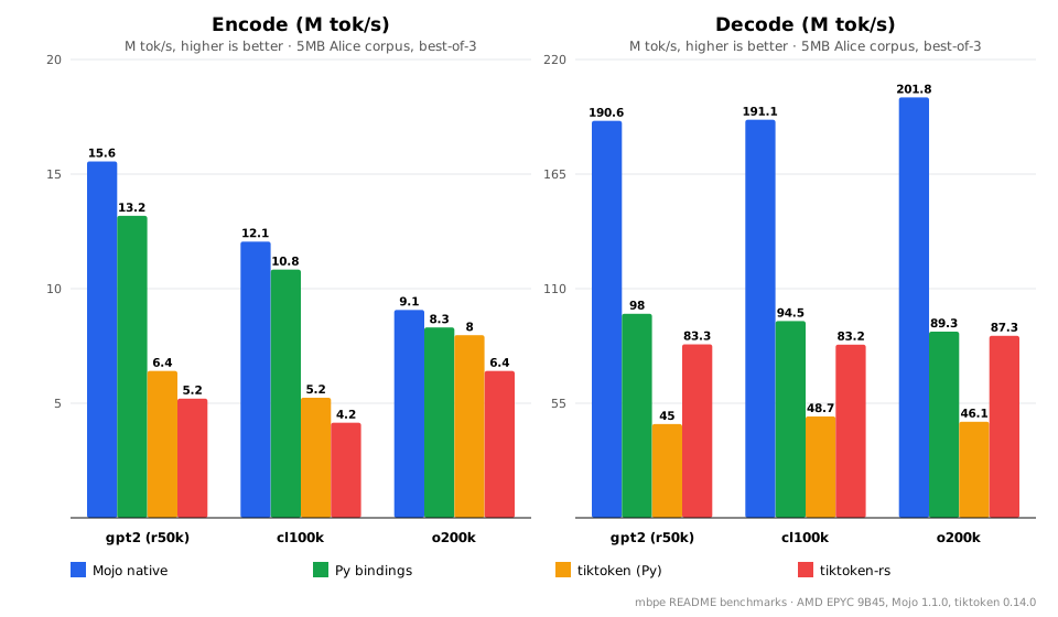
| Encoding | Mojo native | Py bindings | tiktoken (Py) | tiktoken-rs |
|---|---|---|---|---|
| gpt2 (r50k) | 15.9 | 12.1 | 6.3 | 5.9 |
| cl100k | 13.0 | 10.6 | 5.1 | 4.4 |
| o200k | 9.5 | 8.0 | 7.4 | 7.1 |
All units are M tok/s. Bold is the row’s best.
Three observations.
Mojo native is the fastest in every row. The margin over tiktoken is largest on gpt2 (2.5× the Python implementation, 2.7× the Rust one) and narrowest on o200k (1.3× and 1.3×). The o200k vocabulary is the largest of the three and its pre-tokenization rules are more complex, so the encoder does more work per token. The margin shrinks because the baseline is doing more work too — not because mbpe got slower.
The Python bindings are close behind the native path. The gap is roughly 15–25% (narrowest on o200k), which is the cost of crossing the Python/C ABI boundary and constructing Python list objects for the result. Small enough that most Python users will never notice.
Py bindings beat tiktoken (Py) in every row. 1.9× on gpt2, 2.1× on cl100k, 1.1× on o200k. That’s the headline number for anyone replacing tiktoken with mbpe in an existing Python codebase: same API, same .tiktoken files, faster, with no code changes beyond the import.
Decode throughput
| Encoding | Mojo native | Py bindings | tiktoken (Py) | tiktoken-rs |
|---|---|---|---|---|
| gpt2 (r50k) | 199.7 | 92.0 | 44.4 | 85.7 |
| cl100k | 213.0 | 91.0 | 48.0 | 83.2 |
| o200k | 205.5 | 93.5 | 44.5 | 87.8 |
Same units, same bold.
Decode is where §8’s design shows most clearly. Decoding is I/O bound — it reads token bytes and writes them to an output buffer. The flat byte arena makes the read side a linear walk through memory; the single-allocation output string makes the write side a series of unsafe_memcpy calls into one buffer. No pointer chasing, no intermediate allocations.
Mojo native decodes 4–5× faster than tiktoken (Py). On o200k, 205.5 vs. 44.5 — a 4.6× speedup. That’s the largest margin in the chart, and it’s exactly the payoff the arena and single-allocation output were designed for.
Mojo native decodes 2–3× faster than tiktoken-rs. 205.5 vs. 87.8 on o200k — a 2.3× speedup. The Rust implementation is fast, but it doesn’t use a flat arena and doesn’t build the output in one allocation. Those two choices are the difference.
Nothing breaks the sweep. The closest call is gpt2 decode — Py bindings 92.0 vs. tiktoken-rs 85.7 — and it lands on mbpe’s side in this run, as does every other cell: native is fastest in all six rows, and the bindings beat both Python tiktoken and tiktoken-rs in all six.
The Py bindings are slower on decode than on encode, relative to native. 91.0 vs. 213.0 on cl100k — a 2.3× gap. Decoding through Python means constructing a Python str from the Mojo String, which copies every output byte into Python’s heap. Encoding doesn’t pay that: its result is a list of integers, cheap objects next to a whole-string copy. So the ABI overhead is asymmetric. For a Python user, the comparison that matters is Py bindings vs. tiktoken (Py): 91.0 vs. 48.0 on cl100k — 1.9× faster, with no code change.
Why the numbers land where they do
The pattern of speedups maps onto §8’s five layers.
Layers 1 (StringSpan) and 6 (compile-time specialization) affect everything — both encode and decode avoid copying text through owned Strings, and both benefit from the compiler inlining the pre-tokenizer’s logic. This is the baseline speedup running through the whole table.
Layer 2 (flat arena) shows up most in decode. The 4–5× margin there is larger than on encode because decode is where the arena’s memory layout matters most. Encode touches token IDs (integers) in the hot loop; decode touches bytes (in the arena).
Layer 3 (MergeLookup cache) shows up most in encode. Every encode does a pair lookup at every position, and the two-tier lookup table turns most of those into array indexing. The margin is largest on gpt2, where the vocabulary is smallest and the fast path covers the largest fraction of lookups.
Layer 5 (two encode algorithms) shows up on o200k. Its vocabulary has longer merge chains, so words spend more time in the heap-based path — and that path is why the o200k encode margin is still positive despite the extra work.
Layer 4 (incremental pair counts) doesn’t appear in this chart. It’s a training optimization, and these benchmarks are encode/decode on pre-trained vocabularies. Its speedup is real and matters enormously for training, but it’s a different measurement on a different setup.
The environment
AMD EPYC 9B45, 4 cores, 15Gi RAM, Debian GNU/Linux 12 (bookworm). Mojo 1.1.0, Python 3.14.7, Rust 1.99.0, tiktoken 0.14.0.
Performance claims are machine-specific, so the environment is documented. The benchmark is single-threaded — each implementation runs on one core — but the machine’s cache hierarchy and memory bandwidth affect all four implementations the same way. A different machine would change the absolute numbers, not the comparison.
The environment line is regenerated on every run by scripts/update_readme_benchmarks.sh, so the caption is always accurate for the chart it accompanies.
The chart is reproducible
The chart is not hand-drawn. It’s generated by scripts/generate_benchmark_chart.py, which reads JSON-lines result files from benchmarks/results/ and emits the SVG. The flow:
- Run the benchmarks (
bash readme_bench_update.sh), which populatesbenchmarks/results/{native,mbpe,tiktoken,tiktoken-rs}.json. - Run
python3 scripts/generate_benchmark_chart.py, which reads those files and writesdocs/assets/benchmark_chart.svg. - Run
bash scripts/update_readme_benchmarks.sh, which refreshes the environment caption inREADME.md.
The SVG is checked in because it’s embedded in the README, and GitHub renders READMEs but doesn’t run scripts. But it’s not hand-maintained — it’s a rendered output, regenerable by anyone with the same toolchain.
Two properties make the generator pleasant to work with:
- Stdlib only. No matplotlib, no numpy. The SVG is built by string concatenation. Anyone with Python can regenerate the chart, without setting up a visualization environment.
- Deterministic layout. Bar positions, ladder rungs, and axis ceilings are fixed.
nice_maxpicks the first ladder rung that’s at least 8% above the peak value. That’s why the encode axis tops out at 20 and the decode axis tops out at 250. If the numbers don’t change, the SVG doesn’t change — so re-running with unchanged inputs is a no-op diff.
What the benchmarks don’t claim
Not faster on every workload. Short strings or workloads dominated by Python overhead may not see the same speedups. The 5 MB corpus is large enough that per-call overhead is amortized; smaller inputs may see smaller margins.
Not faster than every possible implementation. The baselines are tiktoken and tiktoken-rs, the standard references. A hypothetical hand-tuned C implementation with the same design choices might match or beat mbpe. The claim is narrow: fastest among the implementations compared, on this workload.
Not a training benchmark. Training requires a different setup, a different metric, and a much larger corpus. The training speedup is real — it’s the difference between the incremental pair-count updates and full rescans — but it isn’t measured here. The repository has a separate training benchmark (benchmarks/bm_train.mojo, plus benchmarks/bm_training.mojo for a vocab-size sweep; bash readme_bench_update.sh runs the former into benchmarks/results/training.json), whose numbers are not part of the encode/decode chart above.
Why this matters for the compatibility story
Fast is easy to claim, but hard to prove when you’re also claiming identical output. A fast implementation that produces different token IDs isn’t a fast implementation of the same thing — it’s a fast implementation of a different thing. The benchmark only makes sense if mbpe and tiktoken produce the same IDs on the same input.
They do. The test suite checks byte-for-byte equality on real corpora. All four implementations in the tables above also agreed on token counts — 1,544,948 for gpt2, 1,281,729 for cl100k, 1,277,793 for o200k — and a separate check over a 20,479-byte story came out ID-for-ID identical with zero mismatches on all three vocabularies (5,145 / 4,943 / 4,836 tokens). So the speedup is a speedup on the same work, not on a cheaper variant. Compatibility and speed are not in tension — they’re the two halves of the same claim: mbpe is a correct BPE tokenizer, and it’s fast. The chart is the second half; the test suite is the first.
Five sections of machinery, one question left: does this architecture actually do what it claims? §11 answers the only way that counts — by building a fourth tokenizer, live, end to end, in about thirty lines.
11. One more tokenizer, built live
Ten sections of argument come down to one bet: mbpe is a generic BPE engine, and adding a tokenizer means writing a new PreTokenizer struct, not modifying BPETokenizer. This section collects on that bet by writing one.
The tokenizer we’ll build is a character-level pre-tokenizer. It doesn’t try to match GPT-2’s regex, or any other family’s rules. It splits text into one “word” per codepoint, and that’s the whole rule. The point isn’t that a character-level tokenizer is useful in production — it isn’t, for reasons §2 covered. The point is that the engine doesn’t care. If a pre-tokenizer produces StringSpan views into the input, and provides the trait’s other required pieces, the engine will train, encode, and decode with it exactly as it does with the shipped tokenizers.
The whole pre-tokenizer
Here it is, in full:
from bpe.tokenizer import BPETokenizer, WordCounts
from bpe.pretokenizer import (
    PreTokenizer,
    ByteMapping,
    utf8_codepoint_byte_length,
)

struct CharPretokenizer(PreTokenizer):
    comptime byte_map: ByteMapping = ByteMapping.SEQUENTIAL

    def __init__(out self):
        pass

    @staticmethod
    def name() -> String:
        return String("char")

    def split[
        mut: Bool, //, origin: Origin[mut=mut]
    ](self, text: StringSpan[origin]) raises -> List[StringSpan[origin]]:
        var result = List[StringSpan[origin]]()
        var n = text.byte_length()
        if n == 0:
            return result^
        var span = text.as_bytes()
        var pos = 0
        while pos < n:
            # One "word" per codepoint. Clamp so a truncated trailing
            # sequence never reads past the end.
            var end = pos + utf8_codepoint_byte_length(span[pos])
            if end > n:
                end = n
            result.append(StringSpan(unsafe_from_utf8=span[pos:end]))
            pos = end
        return result^

    def write_to[T: Writer](self, mut writer: T):
        writer.write(String("CharPretokenizer"))
That’s the entire implementation. A required byte_map constant and a required name, the write_to method required by the Writable bound, an overridden split that does the actual work, and a trivial constructor. Everything else comes from trait defaults, each correct for this tokenizer: identity byte mappings (sequential mapping), count_words delegating to split (fine for a toy’s small words), and an empty special_tokens dict.
What the split does
The split method walks the input byte by byte and emits one StringSpan per codepoint. The key step is:
var end = pos + utf8_codepoint_byte_length(span[pos])
utf8_codepoint_byte_length reads the lead byte and returns the total byte length of the codepoint it introduces. It branches on the lead byte’s high bits — <0x80 → 1, <0xE0 → 2, <0xF0 → 3, otherwise 4 — which is how a well-formed lead byte encodes its length. A stray continuation byte (0x80–0xBF) lands in the two-byte branch rather than crashing; the clamp below catches the over-claim. The split then slices span[pos:end] and appends the view.
The if end > n: end = n clamp handles a specific edge case: truncated input. If the last bytes of the input form an incomplete UTF-8 sequence, end would run past the end of the buffer. The clamp prevents that — it doesn’t recover from the malformed input, just keeps the splitter from reading out of bounds. The remainder is emitted as-is, so the pieces still tile the input with no gap and no overlap: the clamp changes the boundary, not the bytes. (The test for this path asserts on the raw split bytes, since the tail doesn’t decode to a valid character.)
Wiring it into the engine
The engine is used exactly as before:
var tok = BPETokenizer[CharPretokenizer]()
That’s the whole wiring: instantiating BPETokenizer with CharPretokenizer gives a fully functional tokenizer — train, encode, encode_ordinary, decode, save_tiktoken, load_tiktoken, everything from §4–§9. The engine doesn’t know it’s character-level; it knows it has a pre-tokenizer. Adding a new tokenizer is writing a struct that satisfies one trait and using it as a type parameter — no change to the training loop, the encode algorithm, the decode path, or the file format.
Does it actually work?
The pre-tokenizer is thirty lines. Before we trust it, we write tests for it. Acceptance criteria: evidence. The tests are how we establish that the pre-tokenizer is wired correctly into the engine, and that the engine really is as pluggable as §7 claimed.
Four checks, each targeting something specific about this pre-tokenizer — the first two are one-liners, the second two get the full treatment.
Split boundaries, in one line. "a中😀" is three codepoints in eight bytes; the splitter must produce three pieces ("a", "中", "😀"), and the test asserts byte_length > piece_count — direct evidence it counts codepoints, not bytes.
Training/encoding agreement, in one line. count_words (the trait default, delegating to split) must report exactly as many entries as split returns pieces on "café中😀" — a regression tripwire for anyone who later overrides count_words with a faster fused version and gets it subtly wrong.
Full pipeline round-trip
This is the test that matters most. It exercises the whole pipeline — split, train, encode, decode — on input that spans four writing systems and three UTF-8 widths:
def test_char_tokenizer_roundtrip_multibyte() raises:
    var tok = BPETokenizer[CharPretokenizer]()
    var corpus = Span[String](
        [
            "café résumé naïve 中文 emoji 😀🎉. In Assamese, the safest approach is"
            " to use the transliterated English term (ক্ল'ষ্ট্ৰ'ফ'বিয়া) or a"
            " descriptive phrase like বন্ধ ঠাইৰ ভয় (fear of closed places)"
        ]
    )
    tok.train(corpus, 300)
    var text = (
        "café 中文 😀 - The single-word terms গুহাতংক and ৰুদ্ধস্থানভীত exist"
    )
    var ids = tok.encode_ordinary(text)
    assert_equal(tok.decode(ids), text)
The training corpus contains Latin text with accented characters (café, résumé, naïve), CJK (中文), emoji (😀🎉), and Assamese script (ক্ল'ষ্ট্ৰ'ফ'বিয়া, বন্ধ ঠাইৰ ভয়). The encode text is a different sentence with the same character classes, including the Assamese terms গুহাতংক and ৰুদ্ধস্থানভীত, which never appeared in training.
The assertion is byte-for-byte equality of the decoded output with the original input. That’s the entire “whole Unicode, exactly” claim from §6, exercised on a real string. If anything in the pipeline is wrong — if split miscounts bytes, if training drops a codepoint, if encode misaligns, if decode loses a byte — the assertion fires. The test would not pass on a tokenizer that was merely byte-level.
No <UNK> on unseen characters
A second round-trip, this time with an emoji that never appeared in training:
def test_char_tokenizer_no_unk_on_unseen_char() raises:
    var tok = BPETokenizer[CharPretokenizer]()
    tok.train(Span[String](["hello world"]), 260)
    var text = "hello 🎉"
    var ids = tok.encode_ordinary(text)
    assert_equal(tok.decode(ids), text)
    text = "Assamese/Hindi ট্ৰাক / ट्रक (ṭrak) ← English truck"
    ids = tok.encode_ordinary(text)
    assert_equal(tok.decode(ids), text)
    text = "Japanese コンピュータ (konpyūta) ← English computer"
    ids = tok.encode_ordinary(text)
    assert_equal(tok.decode(ids), text)
This is the “never emit <UNK>” property made concrete. The training corpus is plain ASCII; the encode text contains an emoji; the round-trip is exact. The emoji decomposes to bytes, the bytes have IDs, the IDs decode back to the bytes, the bytes reassemble to the emoji. No fallback needed, because there’s nothing to fall back to — the byte-level base vocabulary is the fallback.
Two further round-trips on transliterated lines the training corpus never saw extend the same check across scripts — still exact, still no <UNK>. (The real test also round-trips a long multi-script passage, omitted here for length.)
Four checks, then. Two one-liners pin down the splitter’s codepoint-awareness and the training/encoding agreement; two full tests prove the whole pipeline round-trips on input spanning multiple scripts, including characters the training corpus never saw.
Two design choices
Two things about the pre-tokenizer are worth naming, because they’re decisions rather than oversights.
Truncated input. As covered above, the clamp keeps the splitter from reading past the buffer on malformed UTF-8 — but the tail piece doesn’t decode to a valid character. The test asserts on raw bytes rather than the rendered string, which for a truncated tail is an invalid-decoding artifact, not something to depend on.
No special tokens. CharPretokenizer doesn’t declare any. If you wanted to use it with specials, you’d add a special_tokens() override. The default returns an empty dict, which is correct for a character-level tokenizer but worth knowing. The trait doesn’t force either choice.
What the live build demonstrates
The claim §7 made was that adding a tokenizer is writing a new PreTokenizer: a thirty-line struct satisfying the trait (byte_map, name, split), instantiated as BPETokenizer[CharPretokenizer](), then trained, encoded, decoded, saved, and loaded like any shipped tokenizer — with no change to BPETokenizer, the training loop, the encode algorithm, the decode path, or the file format. Building a BPE tokenizer from first principles means writing the algorithm once, then writing one pre-tokenizer per family. The algorithm doesn’t change. Only the front does.
Where this leaves us
That covers problem, algorithm, engine, speed, interfaces, evidence, and extensibility. What remains belongs to no section but the post as a whole: pitfalls, takeaways, and pointers. Those are the appendices.
Common pitfalls (read before you debug)
Six things that will look like bugs but aren’t. Each one is a consequence of a design decision made earlier in the post; each one has bitten someone.
1. Stale _mbpe.so
Python imports the compiled shared library, not the .mojo source files. If you edit bpe/tokenizer.mojo and re-run a Python script, nothing changes — because the script is still loading the .so you built an hour ago.
The fix is to rebuild:
pixi run mojo build python-binding/mbpe.mojo -I . \
    --emit shared-lib -o python-binding/mbpe/_mbpe.so
This is the single most common source of “my fix didn’t work.” The test runner rebuilds from scratch on every run for exactly this reason — you can’t accidentally test against a stale binary.
2. Wrong byte map for o200k
The o200k vocabulary uses a shuffled byte mapping (§6, quirk 1). If you load o200k.tiktoken into a tokenizer whose pre-tokenizer declares ByteMapping.SEQUENTIAL, the file parses successfully — the .tiktoken format doesn’t carry the mapping — but every byte token’s rank is off.
The failure is silent. Encoding a string produces a list of IDs, decoding those IDs produces the same string, and the round-trip test passes. But the IDs aren’t the ones the model was trained against. Downstream, in an actual model, this manifests as garbage output.
Check ByteMapping first. GPT2Pretokenizer and GPT4Pretokenizer[SEQUENTIAL] are sequential; GPT4Pretokenizer[SHUFFLED] is shuffled. The pre-tokenizer’s mapping and the vocabulary file must match.
3. Specials vanish across save/load
By format contract (§9). The .tiktoken file carries only the mergeable vocabulary — special tokens are a type-level property, not a data-level one.
Built-in specials come back automatically after load, because the pre-tokenizer’s special_tokens() declares them (<|endoftext|> for GPT-2, the FIM tokens for cl100k, and so on). Custom specials do not — they must be re-registered by hand after every load:
tok = mbpe.GPT2Tokenizer()
tok.load_tiktoken("my_tokenizer.tiktoken")
tok.register_special_tokens({"<|my_special|>": 50257})
This asymmetry is by design — it makes the file deterministic and diffable, at the cost of not carrying specials — but it’s the most common gotcha in the format.
4. encode vs encode_ordinary
Two methods, two different contracts.
-
encoderecognizes special tokens if they appear in the input. -
encode_ordinarytreats every byte as ordinary text, even if it forms a special token.
If you call encode("<|endoftext|>") and get [50256], and then call encode_ordinary("<|endoftext|>") and get seven tokens ([27, 91, 437, 1659, 5239, 91, 29]) — that’s correct. The seven tokens are the BPE-encoded pieces of the literal string "<|endoftext|>". The single token is the special.
The same applies to the Python wrapper’s allowed_special parameter (§9). An empty allowed-set with disallowed_special="ignore" makes encode behave like encode_ordinary. Seven tokens where you expected one is not a bug — it’s the contract.
5. Data directory mismatch
Two different code paths resolve the data/ directory, and they don’t agree by default.
Mojo side: _find_data_dir in bpe/tokenizer.mojo checks MBPE_DATA_DIR first, falls back to ./data/ relative to the current working directory.
Python side: _find_data_dir in python-binding/mbpe/__init__.py uses importlib.resources to find data/ inside the installed package, with a development fallback relative to the .so’s location.
Setting MBPE_DATA_DIR fixes the Mojo side. It doesn’t fix the Python side, because the Python code doesn’t read that variable. If you’re using both sides and want them to agree, either install the package properly (so importlib.resources finds data/) or keep the repo-root data/ layout the development fallback expects.
6. Forgetting -I .
The bpe/ package resolves only when the Mojo compiler is given -I . — the flag that adds the current directory to the import search path. Without it, from bpe.tokenizer import BPETokenizer fails with a “module not found” error, even if you’re standing in the repository root.
The exception is main.mojo, which Mojo treats as a standalone script and runs without the flag. Everything else — scripts/, tests, the Python binding build — needs it.
Copy invocations from scripts/run_tests.sh rather than writing them from memory. That script has the flags right, and it’s the reason CI doesn’t trip on this.
Takeaways
A language model never sees text. A tokenizer turns text into integer IDs, and only those IDs enter the model. The IDs select embeddings; everything downstream of that lookup — attention, feed-forward, the output projection — operates on vectors, never on text. The tokenizer is the boundary where text and arithmetic meet, and it’s the first and last thing that touches your data.
BPE is a simple algorithm dressed up as a complicated one. Count adjacent pairs. Merge the most frequent. Repeat until you hit a target vocabulary size. Encoding replays the merges in rank order — it never counts. Splitting happens first, and different splitting rules produce different tokenizers even when the merge algorithm is identical.
Subwords are what everyone uses, for three reasons. Bounded vocabulary, so nothing is out-of-vocabulary. Reasonable sequence lengths, so attention doesn’t blow up quadratically. Compositional structure, so the model can generalize from "unhappy" to "unclear" without either word needing to appear whole in training. Byte-level BPE is the specific scheme that makes all three work for any Unicode input.
mbpe is one engine with many fronts. BPETokenizer[PT] is generic over a compile-time pre-tokenizer. GPT-2, GPT-4, and GPT-4o are three instantiations of the same engine, differing only in which PreTokenizer they’re parameterized over. Adding a fourth tokenizer is writing a new struct, not modifying the engine — §11 built one in thirty lines.
The speed comes from identifying costs and eliminating them. Zero-copy StringSpan views instead of owned Strings. A flat byte arena instead of per-token allocations. A two-tier merge lookup table instead of a hash on the hot path. Incremental pair-count updates during training instead of full rescans. Two encode algorithms, selected by word length. Compile-time specialization of the pre-tokenizer so there’s no dispatch in the hot loop. None of these is a trick — each is the standard answer to a specific cost.
Compatibility with tiktoken is a consequence, not a goal. The engine is tiktoken-agnostic; it reads and writes OpenAI’s .tiktoken format because interoperability requires it. The special-token asymmetry, byte-mapping quirks, and r50k_base override are all preserved because matching the ecosystem is what makes the tokenizer useful — and the match is checked, not assumed.
The post opened with eleven characters going in and two integers coming out. Everything since has been about why those two integers are what they are, and what it takes to get them right.
Further reading
The ideas in this post come from a small set of sources, most of them older than the transformer. Here’s where to go if you want to trace them back.
The algorithm. The original BPE paper is Neural Machine Translation of Rare Words with Subword Units by Rico Sennrich, Barry Haddow, and Alexandra Birch (2016). It’s the paper that adapted byte-pair encoding from data compression to subword segmentation for NMT, and it’s the reason GPT-2, GPT-3, GPT-4, and their competitors all use BPE. Short, readable, and the source of the vocabulary-size-vs-coverage framing that §2 gestures at.
The compression origin. BPE itself predates its use in NLP by over two decades. Philip Gage’s 1994 article A New Algorithm for Data Compression in The C Users Journal is the original description of the algorithm as a compression scheme. Reading it is useful for one reason: it makes clear that BPE was never designed for language — it’s a general-purpose byte-pair substitution — and that its success in NLP comes from the fact that text has statistics that BPE happens to exploit well.
The reference implementation. OpenAI’s tiktoken (github.com/openai/tiktoken) is the implementation mbpe is compatible with. Reading its Python and Rust sources is the fastest way to see the same algorithm from a different angle, and it’s the authority on the .tiktoken file format and the OpenAI tokenizer families. If you’re going to use mbpe for anything, you’ll want to know tiktoken too.
The bit tricks. The SWAR helpers in bpe/pretokenizer.mojo — _hasless, _haszero, _letters8 — are standard techniques from Hacker’s Delight by Henry S. Warren, Jr. (§6-1 specifically, on “finding a byte in a word”). The book is worth owning for anyone writing performance-sensitive code; the SWAR chapter in particular is a compact catalog of things you can do with a 64-bit register that look like they shouldn’t be possible. SWAR.md traces how these three helpers work and why mbpe chose them over Mojo’s SIMD type.
Unicode properties. The class table in bpe/unicode_tables.mojo is generated from Python’s regex module, which tracks the Unicode Character Database. The UCD itself (unicode.org/Public/UCD/latest/) is the ground truth for what counts as a letter, a digit, or whitespace — the property definitions the generator consumes. If you ever disagree with the table, the UCD is where you go to find out who’s wrong.
The SWAR ancestry. The technique of treating a register as a vector of narrow lanes — which is what _hasless and _haszero do — has a long history outside compression, in everything from cryptographic implementations to string search. If the idiom feels alien, it’s worth spending an afternoon reading a modern SIMD tutorial and then re-reading §6’s Unicode section; the pattern-matching instinct for what fits in a register will serve you more broadly than just this project.
The code. Everything discussed here lives at github.com/ratulb/mbpe. The README has install instructions, benchmark reproduction steps, and the same chart that appears in §10. scripts/run_tests.sh is the canonical way to run the test suite; the benchmarks/ directory has the benchmark scripts; and docs/assets/benchmark_chart.svg is the generated chart embedded in §10. If you want to extend the engine — write a new pre-tokenizer, add a new encoding family, or port a piece of it to another language — the code is the place to start, and the source files are commented at the level of detail that this post tries to match.
One last thing
The post has argued that mbpe is a correct and fast BPE tokenizer, and that it’s built on a generic engine with pluggable front ends. That claim is only as good as the code, and the code is only as good as the tests that guard it.
The interesting part of a tokenizer isn’t the algorithm, it’s the discipline of getting the edge cases right. The rank invariant that makes merge recovery possible. The byte-mapping distinction between sequential and shuffled. The Unicode property table that has to be right for every codepoint, not just the ones you thought to test. The special-token asymmetry that falls out of a format decision. None of these are hard to state, and every one of them is easy to get wrong.
That’s the work. The algorithm fits on a page. The correctness is where the pages go.