<?xml version="1.0" encoding="utf-8"?><feed xmlns="http://www.w3.org/2005/Atom" ><generator uri="https://jekyllrb.com/" version="3.10.0">Jekyll</generator><link href="https://ratulb.github.io/techcottage/feed.xml" rel="self" type="application/atom+xml" /><link href="https://ratulb.github.io/techcottage/" rel="alternate" type="text/html" /><updated>2026-07-03T16:26:39+00:00</updated><id>https://ratulb.github.io/techcottage/feed.xml</id><title type="html">Tech Cottage</title><subtitle>Mojo, Tenmo, Rust, Kubernetes, and systems programming</subtitle><author><name>rbsomeg</name></author><entry><title type="html">From Bytes to Gradients: Tracing a Neural Network Through Tenmo, One Layer at a Time</title><link href="https://ratulb.github.io/techcottage/2026/06/from-bytes-to-gradients/" rel="alternate" type="text/html" title="From Bytes to Gradients: Tracing a Neural Network Through Tenmo, One Layer at a Time" /><published>2026-06-30T00:00:00+00:00</published><updated>2026-06-30T00:00:00+00:00</updated><id>https://ratulb.github.io/techcottage/2026/06/from-bytes-to-gradients</id><content type="html" xml:base="https://ratulb.github.io/techcottage/2026/06/from-bytes-to-gradients/"><![CDATA[<p>When you call <code class="language-plaintext highlighter-rouge">loss.backward()</code> in PyTorch, a C++ autograd engine climbs the computation graph in reverse, multiplying Jacobians until every leaf tensor has its gradient filled in. It works. It’s fast. But the graph lives in C++ libraries you never see — <code class="language-plaintext highlighter-rouge">torch::autograd::Engine</code>, <code class="language-plaintext highlighter-rouge">THPVariable</code>, <code class="language-plaintext highlighter-rouge">VariableType</code> — hundreds of thousands of lines built over a decade.</p>

<p>What if you could read <em>every line</em> of the system between <code class="language-plaintext highlighter-rouge">loss.backward()</code> and the weight update? That’s the premise of Tenmo, a tensor library and neural network framework written entirely in Mojo. Every autograd dispatch, every SIMD matmul kernel, every GPU launch is in one repository under 100 source files.</p>

<p>This post traces one MNIST training step — <code class="language-plaintext highlighter-rouge">matmul → bias_add → relu → matmul → bias_add → relu → matmul → bias_add → cross_entropy</code> — through every layer of the system. We’ll start with raw memory allocation and end with the final parameter update, showing the real code at each stage.</p>

<h2 id="1-the-memory-model--buffer">1. The Memory Model — Buffer</h2>

<p>Every tensor operation eventually reads or writes a flat array of scalars. In Tenmo, that flat array is a <code class="language-plaintext highlighter-rouge">Buffer[dtype]</code> — a CPU-only, shape-agnostic block of memory with one optional feature: reference counting.</p>

<pre><code class="language-mojo">struct Buffer[dtype: DType = DType.float32]:
    var size: Int
    var data: Optional[UnsafePointer[Scalar[Self.dtype], MutAnyOrigin]]
    var _refcount: Optional[UnsafePointer[Atomic[DType.uint64], MutAnyOrigin]]
    var external: Bool
</code></pre>

<p>A <code class="language-plaintext highlighter-rouge">Buffer</code> has two modes. <strong>Unshared</strong>: a single allocated block of <code class="language-plaintext highlighter-rouge">Scalar[dtype]</code> elements with no reference counting. <code class="language-plaintext highlighter-rouge">__init__(*, copy:)</code> deep-copies the data — malloc + memcpy. <strong>Shared</strong>: the allocation layout is <code class="language-plaintext highlighter-rouge">[refcount: Atomic(UInt64)] | [data array]</code>, and <code class="language-plaintext highlighter-rouge">__init__(*, copy:)</code> merely bumps the atomic counter. <code class="language-plaintext highlighter-rouge">__del__</code> decrements; when it hits zero, the combined allocation is freed in one shot.</p>

<p>The <code class="language-plaintext highlighter-rouge">shared()</code> method transforms an unshared buffer in-place (line 122 of <code class="language-plaintext highlighter-rouge">buffers.mojo</code>):</p>

<pre><code class="language-mojo">def shared(mut self):
    if self.is_shared():
        return
    var refcount_size = size_of[Atomic[DType.uint64]]()
    var data_size = self.size * size_of[Scalar[Self.dtype]]()
    var total_size = refcount_size + data_size
    var new_alloc = alloc[UInt8](total_size)
    var refcount_ptr = new_alloc.bitcast[Atomic[DType.uint64]]()
    refcount_ptr[] = Atomic[DType.uint64](1)
    var new_data = (new_alloc + refcount_size).bitcast[Scalar[Self.dtype]]()
    memcpy(dest=new_data, src=self.data, count=self.size)
    self.data.unsafe_value().free()
    self.data = new_data
    self._refcount = refcount_ptr
</code></pre>

<p>This allocation layout matters because views share the same Buffer via refcount bump. When we slice a tensor, the new tensor’s NDBuffer points to the same underlying Buffer with a refcount of 2. The memory stays alive as long as any view holds a reference, regardless of Mojo’s aggressive destruction of intermediate tensors.</p>

<p>There’s also a static <code class="language-plaintext highlighter-rouge">Buffer.shared(size)</code> constructor that allocates the combined layout from the start, avoiding the O(n) reallocation that the instance <code class="language-plaintext highlighter-rouge">shared()</code> method performs. This is the fast path used by <code class="language-plaintext highlighter-rouge">Gradbox.__init__</code>.</p>

<h2 id="2-shape--strides--views--ndbuffer">2. Shape + Strides + Views — NDBuffer</h2>

<p>A flat Buffer doesn’t know about dimensions. That’s the job of <code class="language-plaintext highlighter-rouge">NDBuffer[dtype]</code> — the single source of truth for shape, strides, offset, and device location.</p>

<pre><code class="language-mojo">struct NDBuffer[dtype: DType]:
    var shape: Shape
    var strides: Strides
    var offset: Int
    var _contiguous: Bool
    var buffer: Buffer[dtype]      # CPU data
    var device_state: Optional[DeviceState]  # GPU data
</code></pre>

<p>The key insight: <code class="language-plaintext highlighter-rouge">NDBuffer</code> doesn’t own the data. It points into a <code class="language-plaintext highlighter-rouge">Buffer</code> at some <code class="language-plaintext highlighter-rouge">offset</code>, interpreting the flat memory through <code class="language-plaintext highlighter-rouge">strides</code>. A contiguous tensor <code class="language-plaintext highlighter-rouge">(3, 4)</code> with strides <code class="language-plaintext highlighter-rouge">(4, 1)</code> and offset <code class="language-plaintext highlighter-rouge">0</code> maps element <code class="language-plaintext highlighter-rouge">(i, j)</code> to <code class="language-plaintext highlighter-rouge">buffer[i*4 + j]</code>. A transposed view of the same tensor has strides <code class="language-plaintext highlighter-rouge">(1, 4)</code> and offset <code class="language-plaintext highlighter-rouge">0</code> — element <code class="language-plaintext highlighter-rouge">(i, j)</code> maps to <code class="language-plaintext highlighter-rouge">buffer[i*1 + j*4]</code>.</p>

<p>Zero-copy slicing uses <code class="language-plaintext highlighter-rouge">share()</code>:</p>

<pre><code class="language-mojo">def share(
    self, new_shape: Shape, new_strides: Strides, new_offset: Int
) -&gt; NDBuffer[Self.dtype]:
    # Enables refcounting on the CPU Buffer (first call does the transform)
    self.buffer.shared()
    # Returns a new NDBuffer pointing at the same Buffer
    return NDBuffer(...)
</code></pre>

<p>On GPU, there’s no separate sharing step — <code class="language-plaintext highlighter-rouge">DeviceBuffer</code> (Mojo’s GPU built-in) is always refcounted. The <code class="language-plaintext highlighter-rouge">device_state</code> is simply copied by pointer.</p>

<p><code class="language-plaintext highlighter-rouge">reshape()</code> exploits this: if the new shape’s <code class="language-plaintext highlighter-rouge">max_index</code> fits within the underlying <code class="language-plaintext highlighter-rouge">buffer_size</code>, it returns a zero-copy view with new strides and offset. Only when the view would require discontiguous access does it materialize a contiguous copy.</p>

<p>This is the foundation for the “reshape is free” property of the autograd graph. A <code class="language-plaintext highlighter-rouge">ReshapeBackward</code> handler (in <code class="language-plaintext highlighter-rouge">reshape.mojo</code>) does nothing but reshape the gradient tensor to the parent’s shape — no data transformation, just a new <code class="language-plaintext highlighter-rouge">Shape</code> and <code class="language-plaintext highlighter-rouge">Strides</code> object.</p>

<h2 id="3-tensor--the-user-facing-type">3. Tensor — The User-Facing Type</h2>

<p>The <code class="language-plaintext highlighter-rouge">Tensor[dtype]</code> struct bundles an NDBuffer with autograd metadata:</p>

<pre><code class="language-mojo">struct Tensor[dtype: DType]:
    var _id: UInt
    var buffer: NDBuffer[Self.dtype]
    var requires_grad: Bool
    var gradbox: Optional[Gradbox[Self.dtype]]
    var ancestors: Optional[Ancestors[Self.dtype]]
</code></pre>

<p>Two of these fields deserve a closer look.</p>

<p><strong>Gradbox</strong> — this is not Tensor, and that matters. Tensor is 4543 lines of code; Gradbox is 1526. Gradbox doesn’t need  reductions, trig, comparisons, or many of the 200-odd operations Tensor supports. It only needs gradient storage shapes, accumulation (add, subtract, zero), reshape, broadcast, and device transfer. That’s it. A lean container specialized for one job.</p>

<p>Technically, Gradbox is a combined heap allocation of <code class="language-plaintext highlighter-rouge">[Atomic(UInt64)] | [NDBuffer]</code>. The atomic refcount is <em>independent</em> of the Tensor’s refcount. When Mojo’s ASAP destruction drops an intermediate tensor, the Gradbox survives if other handles (Ancestor copies in the graph) still reference it. This prevents dangling pointers in the autograd graph.</p>

<pre><code class="language-mojo">struct Gradbox[dtype: DType]:
    var _ndb_ptr: Optional[UnsafePointer[NDBuffer, MutAnyOrigin]]
    var _refcount: Optional[UnsafePointer[Atomic[DType.uint64], MutAnyOrigin]]
</code></pre>

<p>In <code class="language-plaintext highlighter-rouge">__init__(shape)</code> (line 33 of <code class="language-plaintext highlighter-rouge">gradbox.mojo</code>), it allocates one block, initializes the atomic to 1, and constructs the NDBuffer via move-init. <code class="language-plaintext highlighter-rouge">__init__(*, copy:)</code> bumps the atomic via <code class="language-plaintext highlighter-rouge">fetch_add[RELAXED](1)</code>. <code class="language-plaintext highlighter-rouge">__del__</code> decrements via <code class="language-plaintext highlighter-rouge">fetch_sub[RELEASE](1)</code>; if the result is 1 (meaning this was the last handle), it destroys the NDBuffer and frees the combined allocation.</p>

<p>When you need to convert between the two, <code class="language-plaintext highlighter-rouge">Gradbox.as_tensor()</code> (<code class="language-plaintext highlighter-rouge">gradbox.mojo:118</code>) materializes a contiguous copy of the gradient data as a Tensor, and <code class="language-plaintext highlighter-rouge">Tensor.as_gradbox()</code> (<code class="language-plaintext highlighter-rouge">tensor.mojo:135</code>) consumes the Tensor’s NDBuffer to produce a Gradbox. This metamorphosis between types is explicit — you don’t accidentally use a gradient storage container as a full tensor.</p>

<p><strong>Ancestor</strong> — The old Tenmo design stored full <code class="language-plaintext highlighter-rouge">Tensor</code> copies at every <code class="language-plaintext highlighter-rouge">add_ancestry</code> call, triggering recursive deep copies, gradbox allocations, and heap blocks. The current design uses a lightweight handle:</p>

<pre><code class="language-mojo">struct Ancestor[dtype: DType]:
    var _id: UInt
    var requires_grad: Bool
    var gradbox: Optional[Gradbox[Self.dtype]]
    var ndb: Optional[NDBuffer[Self.dtype]]
    var parents: Optional[Ancestors[Self.dtype]]
</code></pre>

<p>The <code class="language-plaintext highlighter-rouge">ndb</code> field is only populated when <code class="language-plaintext highlighter-rouge">needs_parent_data=True</code> — most operations don’t need it. Addition doesn’t need the parent’s buffer; it just passes the gradient through unchanged. Matmul does need the parent’s data (to compute <code class="language-plaintext highlighter-rouge">grad × B^T</code>), so <code class="language-plaintext highlighter-rouge">needs_parent_data=True</code> is set on its <code class="language-plaintext highlighter-rouge">BackwardFnArg</code>.</p>

<h2 id="4-forward-pass--a-real-mnist-step">4. Forward Pass — A Real MNIST Step</h2>

<p>With the data structures in hand, let’s trace one batch through the MNIST model. The architecture is <code class="language-plaintext highlighter-rouge">784 → 128 → ReLU → 32 → ReLU → 10</code>, built as a <code class="language-plaintext highlighter-rouge">Sequential</code>:</p>

<pre><code class="language-mojo">var model = Sequential[dtype]()
model.append(
    Linear[dtype](784, 128).into(),
    ReLU[dtype]().into(),
    Linear[dtype](128, 32).into(),
    ReLU[dtype]().into(),
    Linear[dtype](32, 10).into(),
)
</code></pre>

<p>A forward call <code class="language-plaintext highlighter-rouge">model(x)</code> dispatches through each layer in sequence. The heaviest operation by far is <code class="language-plaintext highlighter-rouge">matmul</code> — three of them per batch, each computing <code class="language-plaintext highlighter-rouge">(batch_size, in_features) × (in_features, out_features)</code>.</p>

<h3 id="matmul--the-cpu-kernel">Matmul — The CPU Kernel</h3>

<p>The CPU matmul lives in <code class="language-plaintext highlighter-rouge">matmul_cpu.mojo</code>, struct <code class="language-plaintext highlighter-rouge">MmCpu2d</code>. It selects from 18 tile configurations based on the matrix dimensions (<code class="language-plaintext highlighter-rouge">m</code>, <code class="language-plaintext highlighter-rouge">n</code>, <code class="language-plaintext highlighter-rouge">p</code>):</p>

<pre><code class="language-mojo">var tile_m = 128 if m &gt; 256 else (64 if m &gt; 64 else 32)
var tile_n = 64  if n &gt; 64  else 32
var tile_p = 256 if p &gt; 256 else (128 if p &gt; 64 else 64)
</code></pre>

<p>For the first layer <code class="language-plaintext highlighter-rouge">(64, 784) × (784, 128)</code>, <code class="language-plaintext highlighter-rouge">m=64, n=784, p=128</code>. Tracing through the selection (matmul_cpu.mojo:87–89):</p>

<ul>
  <li><code class="language-plaintext highlighter-rouge">tile_m = 128 if m &gt; 256 else (64 if m &gt; 64 else 32)</code> — <code class="language-plaintext highlighter-rouge">m=64</code>: <code class="language-plaintext highlighter-rouge">64 &gt; 256</code> false → <code class="language-plaintext highlighter-rouge">64 &gt; 64</code> false → <strong>tile_m=32</strong></li>
  <li><code class="language-plaintext highlighter-rouge">tile_n = 64 if n &gt; 64 else 32</code> — <code class="language-plaintext highlighter-rouge">n=784 &gt; 64</code> → <strong>tile_n=64</strong></li>
  <li><code class="language-plaintext highlighter-rouge">tile_p = 256 if p &gt; 256 else (128 if p &gt; 64 else 64)</code> — <code class="language-plaintext highlighter-rouge">p=128</code>: <code class="language-plaintext highlighter-rouge">128 &gt; 256</code> false → <code class="language-plaintext highlighter-rouge">128 &gt; 64</code> true → <strong>tile_p=128</strong></li>
</ul>

<p>Result: <code class="language-plaintext highlighter-rouge">MmCpu2d[float32, 32, 64, 128]</code> — the <code class="language-plaintext highlighter-rouge">tile_m=32</code> branch of the 18-way dispatch table.</p>

<p>Note the <code class="language-plaintext highlighter-rouge">tile_p=128</code> choice. The <code class="language-plaintext highlighter-rouge">p &gt; 64</code> check that picks 128 over 256 when <code class="language-plaintext highlighter-rouge">p=128</code> is about L1 cache capacity, not SIMD utilization. Tile_P controls the outer <code class="language-plaintext highlighter-rouge">j_tile</code> stride — how many columns of B are loaded per <code class="language-plaintext highlighter-rouge">k_tile</code> pass and reused across all rows in the tile. With <code class="language-plaintext highlighter-rouge">TILE_N=64</code> and <code class="language-plaintext highlighter-rouge">TILE_P=256</code>, the B j-tile is <code class="language-plaintext highlighter-rouge">64 × 256 × 4 bytes = 64 KB</code>, which overflows L1 data cache (32 KB). With <code class="language-plaintext highlighter-rouge">TILE_P=128</code>, it’s <code class="language-plaintext highlighter-rouge">64 × 128 × 4 = 32 KB</code>, fitting perfectly. The inner SIMD unrolled loop (32 columns per iteration) is equally efficient in either case — <code class="language-plaintext highlighter-rouge">j_end = min(j_tile + TILE_P, p)</code> caps it at the actual 128 columns regardless of <code class="language-plaintext highlighter-rouge">TILE_P</code>, so 4 iterations of 32 columns fully cover the output with no tail.</p>

<p>Inside the selected tile configuration, the hot loop processes columns in groups of <code class="language-plaintext highlighter-rouge">simd_unroll = simdwidth × UNROLL</code> (for float32 with AVX2: <code class="language-plaintext highlighter-rouge">8 × 4 = 32</code> columns per iteration):</p>

<pre><code class="language-mojo"># Unrolled SIMD: 4 independent accumulators fill the FMA pipeline
var acc0: SIMD[Self.dtype, simdwidth]
var acc1: SIMD[Self.dtype, simdwidth]
var acc2: SIMD[Self.dtype, simdwidth]
var acc3: SIMD[Self.dtype, simdwidth]

if k_tile == 0:
    acc0 = SIMD[Self.dtype, simdwidth](0)  # C is zeroed, skip load
else:
    acc0 = C_data.load[width=simdwidth](cj)

for k in range(k_tile, k_end):
    var a_ik = SIMD[Self.dtype, simdwidth](A_data[a_row_base + k])
    var b_base = k * B_stride0 + B_offset + j
    acc0 = math.fma(a_ik, B_data.load[width=simdwidth](b_base), acc0)
    acc1 = math.fma(a_ik, B_data.load[width=simdwidth](b_base + simdwidth), acc1)
    acc2 = math.fma(a_ik, B_data.load[width=simdwidth](b_base + simdwidth * 2), acc2)
    acc3 = math.fma(a_ik, B_data.load[width=simdwidth](b_base + simdwidth * 3), acc3)
</code></pre>

<p>Each iteration: one broadcast of <code class="language-plaintext highlighter-rouge">a_ik</code> (scalar→SIMD), four SIMD loads from B, four FMA instructions. For float32 with <code class="language-plaintext highlighter-rouge">simdwidth=8</code>: <strong>32 FMAs per inner iteration</strong>. The <code class="language-plaintext highlighter-rouge">k_tile==0</code> optimization skips loading C (it starts zeroed), saving 4 vector reads on the first tile pass.</p>

<p>Rows are parallelized across physical cores using <code class="language-plaintext highlighter-rouge">parallelize</code> from Mojo’s standard library — each core processes a contiguous block of <code class="language-plaintext highlighter-rouge">TILE_M</code> rows with its own cache-hot k-strip and j-tile.</p>

<h3 id="bias-add--broadcast-arithmetic">Bias Add — Broadcast Arithmetic</h3>

<p>After matmul, bias addition broadcasts a <code class="language-plaintext highlighter-rouge">(128,)</code> vector across the batch dimension. This dispatches through <code class="language-plaintext highlighter-rouge">CpuArithmeticOps.broadcast</code> (<code class="language-plaintext highlighter-rouge">cpu_arithmetics.mojo</code>) which selects Tier 2: one operand has unit stride in the last dimension, the other broadcasts (stride 0).</p>

<pre><code class="language-mojo"># Tier 2: SIMD splat from broadcasting side
var scalar_vec = SIMD[Self.dtype, simd_width](scalar_v)
while j + simd_width &lt;= last_dim:
    var vec = b.buffer.load[simdwidth=simd_width](b_off + j)
    var op_result = simd_op[op_code, Self.dtype, simd_width](vec, scalar_vec)
    buffer.store[simdwidth=simd_width](out_base + j, op_result)
    j += simd_width
</code></pre>

<p>A single scalar is splatted into a SIMD register, then the contiguous side is SIMD-loaded and vector-added. This is the same mechanism used by every broadcasting op in the system — bias add, layer norm, cross-entropy sub-ops.</p>

<h3 id="cross-entropy--fused-gpu-kernel">Cross-Entropy — Fused GPU Kernel</h3>

<p>The final layer produces logits <code class="language-plaintext highlighter-rouge">(64, 10)</code>. <code class="language-plaintext highlighter-rouge">CrossEntropyLoss</code> dispatches through <code class="language-plaintext highlighter-rouge">CrossEntropyFusedKernel</code> on GPU (at <code class="language-plaintext highlighter-rouge">tenmo/kernels/crossentropy_fused_kernel.mojo</code>). This fused kernel computes max-reduce, exp, sum-exp, softmax, and NLL in a single GPU launch:</p>

<ul>
  <li>Thread-block-per-row pattern (M = 64 blocks)</li>
  <li>Shared-memory tree reduction for max and sum_exp</li>
  <li>Register-level log_softmax computation</li>
  <li>Single scalar write per block for the loss value</li>
</ul>

<p>Without this fusion, <code class="language-plaintext highlighter-rouge">cross_entropy</code> would trigger ~18 separate kernel launches plus a CPU onehot fallback. The fused kernel reduces it to 1 launch + 4 backward arithmetic ops.</p>

<p>On CPU, cross-entropy uses an analogous fused path that walks rows with SIMD vectorization, computing the max, exp, sum, log, and NLL in a single row loop.</p>

<h2 id="5-the-backward-graph">5. The Backward Graph</h2>

<p>Every forward operation that needs gradient tracking registers a <code class="language-plaintext highlighter-rouge">BackwardFnArg</code> and parent <code class="language-plaintext highlighter-rouge">Ancestor</code> handles on the output tensor. Let’s see what happens when we call <code class="language-plaintext highlighter-rouge">loss.backward()</code>.</p>

<h3 id="what-add_ancestry-stores">What <code class="language-plaintext highlighter-rouge">add_ancestry</code> Stores</h3>

<p>When <code class="language-plaintext highlighter-rouge">Multiplicator.forward()</code> registers <code class="language-plaintext highlighter-rouge">c = a * b</code>, it creates:</p>

<pre><code class="language-mojo">var backwardFnArg = BackwardFnArg[Self.dtype].null_arg(BACKWARD_MULTIPLY)
backwardFnArg.needs_parent_data = True  # backward needs parent buffer
out.add_ancestry(backwardFnArg^, self, other)
</code></pre>

<p>The <code class="language-plaintext highlighter-rouge">BackwardFnArg</code> is the dispatch key — a type-erased container packing the integer <code class="language-plaintext highlighter-rouge">op_code</code> together with a destructor function and copier function for whatever payload it carries. The 58 operation codes are defined as <code class="language-plaintext highlighter-rouge">comptime</code> constants in <code class="language-plaintext highlighter-rouge">backpropagation.mojo</code> (e.g. <code class="language-plaintext highlighter-rouge">BACKWARD_ADD = 0</code>, <code class="language-plaintext highlighter-rouge">BACKWARD_MATMUL_2D = 4</code>, <code class="language-plaintext highlighter-rouge">BACKWARD_SIGMOID = 7</code>).</p>

<p><code class="language-plaintext highlighter-rouge">add_ancestry()</code> (<code class="language-plaintext highlighter-rouge">tensor.mojo:1080</code>) converts each parent Tensor into an <code class="language-plaintext highlighter-rouge">Ancestor</code> handle. When <code class="language-plaintext highlighter-rouge">needs_parent_data=True</code>, it copies the parent’s NDBuffer and calls <code class="language-plaintext highlighter-rouge">buffer.share()</code> to enable refcounting. When <code class="language-plaintext highlighter-rouge">False</code> (most ops), it creates the ancestor with no ndb — just the <code class="language-plaintext highlighter-rouge">_id</code>, <code class="language-plaintext highlighter-rouge">requires_grad</code> flag, and gradbox pointer.</p>

<h3 id="the-backward-pass--phase-by-phase">The Backward Pass — Phase by Phase</h3>

<p>The <code class="language-plaintext highlighter-rouge">backward()</code> method at <code class="language-plaintext highlighter-rouge">tensor.mojo:3160</code> proceeds in three phases:</p>

<p><strong>Phase 1: Seed gradient.</strong> <code class="language-plaintext highlighter-rouge">output.seed_grad(1.0)</code> allocates the output’s gradbox (if needed) and fills it with 1.0. On GPU, <code class="language-plaintext highlighter-rouge">sync=True</code> fences all pending GPU work before the seed — ensuring forward kernel outputs are visible before backward reads them.</p>

<p><strong>Phase 2: DFS graph collection.</strong> Starting from the output’s <code class="language-plaintext highlighter-rouge">Ancestor</code>, the code walks parent references recursively, building three parallel structures:</p>

<pre><code class="language-mojo">var node_list = List[Ancestor[Self.dtype]]
var fanin = Dict[UInt, Int]()
var id_to_index = Dict[UInt, Int]()

# DFS: push root, pop, visit parents
var root = output.to_ancestor()
root.ndb = output.buffer.copy()  # root always gets data
dfs_stack.append(root._id)
while len(dfs_stack) &gt; 0:
    var node_id = dfs_stack.pop()
    if node_id in visited:
        continue
    visited.add(node_id)
    topo_ids.append(node_id)
    if node.has_ancestry():
        for parent in node.ancestry():
            var parent_id = parent._id
            fanin[parent_id] = fanin.get(parent_id, 0) + 1
            if parent_id not in id_to_index:
                node_list.append(parent.copy())
                id_to_index[parent_id] = new_idx
                dfs_stack.append(parent_id)
</code></pre>

<p><code class="language-plaintext highlighter-rouge">fanin</code> counts how many children depend on each node. The root has fanin 0. A matmul node may have fanin 0 (no one depends on its gradient) or 1 (a ReLU sits on top).</p>

<p><strong>Phase 3: Reverse topological execution.</strong> A <code class="language-plaintext highlighter-rouge">ready_queue</code> starts with the root. For each popped node:</p>

<ol>
  <li><code class="language-plaintext highlighter-rouge">Backward.invoke(node, parent_ids)</code> dispatches via a 58-way jump table on <code class="language-plaintext highlighter-rouge">op_code</code> to the appropriate backward handler</li>
  <li>The handler reads <code class="language-plaintext highlighter-rouge">output.gradients()</code>, computes parent gradient contributions, calls <code class="language-plaintext highlighter-rouge">parent.update_grad(grad, op_code, extra_arg)</code> to accumulate into each parent’s gradbox</li>
  <li>For each parent that received gradient, its <code class="language-plaintext highlighter-rouge">_id</code> is appended to <code class="language-plaintext highlighter-rouge">parent_ids</code></li>
  <li>Each parent’s fanin is decremented; when it hits 0 and the parent has ancestry, it’s enqueued</li>
</ol>

<h3 id="example-multiply-broadcast-backward">Example: Multiply Broadcast Backward</h3>

<p>When <code class="language-plaintext highlighter-rouge">c = a * b</code> with broadcasting (e.g. <code class="language-plaintext highlighter-rouge">a</code> is <code class="language-plaintext highlighter-rouge">(3, 1)</code> and <code class="language-plaintext highlighter-rouge">b</code> is <code class="language-plaintext highlighter-rouge">(1, 4)</code>), the backward handler at <code class="language-plaintext highlighter-rouge">multiplication.mojo:85</code> is aliased to <code class="language-plaintext highlighter-rouge">BroadcastBackward</code>. This handler:</p>

<ol>
  <li>Extracts the upstream gradient <code class="language-plaintext highlighter-rouge">∂loss/∂c</code> from the output’s gradbox</li>
  <li>Broadcasts/unbroadcasts it to each parent’s shape</li>
  <li>If the op is multiplication, scales by the other parent’s values: <code class="language-plaintext highlighter-rouge">∂loss/∂a = ∂loss/∂c * b</code></li>
  <li>Calls <code class="language-plaintext highlighter-rouge">ancestor.update_grad(grad_contrib, AddTensor, None)</code> for each parent</li>
</ol>

<p>The <code class="language-plaintext highlighter-rouge">update_grad</code> method at <code class="language-plaintext highlighter-rouge">ancestry.mojo:72</code> dispatches on the <code class="language-plaintext highlighter-rouge">op_code</code> parameter:</p>
<ul>
  <li><code class="language-plaintext highlighter-rouge">AddTensor</code>: <code class="language-plaintext highlighter-rouge">gradbox += incoming</code> (in-place addition)</li>
  <li><code class="language-plaintext highlighter-rouge">ScatterAddTensor</code>: <code class="language-plaintext highlighter-rouge">Filler.scatter_add()</code> for sparse gradient accumulation (used by Gather backward)</li>
  <li><code class="language-plaintext highlighter-rouge">ZeroGrad</code>: <code class="language-plaintext highlighter-rouge">gradbox.zero_grad()</code></li>
</ul>

<h3 id="the-aha-moment--reshape-backward">The “Aha” Moment — Reshape Backward</h3>

<p><code class="language-plaintext highlighter-rouge">ReshapeBackward</code> (<code class="language-plaintext highlighter-rouge">reshape.mojo:13</code>) is the simplest backward in the system:</p>

<pre><code class="language-mojo">def backward(output, mut parent_ids, retain_graph=False):
    ref gradbox = output.gradients()
    var ancestor = output.ancestry().get(0)
    if ancestor.requires_grad:
        var reshaped = gradbox.reshape(ancestor.shape())
        ancestor.update_grad(reshaped^, AddTensor, None)
</code></pre>

<p>It just reshapes the gradient tensor to the parent’s shape. No data transformation — a new <code class="language-plaintext highlighter-rouge">Shape</code> and <code class="language-plaintext highlighter-rouge">Strides</code> object, same Buffer, same values. If your forward was <code class="language-plaintext highlighter-rouge">(2,6) → reshape(3,4)</code>, backward is just <code class="language-plaintext highlighter-rouge">gradient(3,4) → reshape(2,6)</code>. The gradient values pass through unchanged.</p>

<p>This contradicts the naive intuition that “reshape is a math op that rearranges data”. It’s a metadata op. The backward proves it.</p>

<h2 id="6-the-optimizer--sgd-step">6. The Optimizer — SGD Step</h2>

<p>After backward fills every gradient, <code class="language-plaintext highlighter-rouge">SGD.step()</code> updates the parameters. The optimizer struct at <code class="language-plaintext highlighter-rouge">optim.mojo:10</code> holds pointers to parameters, velocity buffers (for momentum), and hyperparameters.</p>

<pre><code class="language-mojo">struct SGD[dtype: DType, //]:
    var parameters: List[UnsafePointer[Tensor[Self.dtype], MutAnyOrigin]]
    var lr: Scalar[Self.dtype]
    var momentum: Scalar[Self.dtype]
    var weight_decay: Scalar[Self.dtype]
    var velocities: List[Gradbox[Self.dtype]]
</code></pre>

<p>The <code class="language-plaintext highlighter-rouge">step()</code> method iterates each parameter, checks <code class="language-plaintext highlighter-rouge">requires_grad &amp;&amp; has_grad()</code>, and runs the update. On CPU, it’s SIMD-vectorized:</p>

<pre><code class="language-mojo">def _step_no_momentum[simd_w: Int](self, param_ptr, grad_ptr, num_elements):
    var lr_vec = SIMD[Self.dtype, simd_w](self.lr)
    var wd_vec = SIMD[Self.dtype, simd_w](self.weight_decay)
    for j in range(0, vec_end, simd_w):
        var p_vec = param_ptr.load[width=simd_w](j)
        var g_vec = grad_ptr.load[width=simd_w](j)
        if self.weight_decay &gt; 0:
            g_vec += p_vec * wd_vec
        p_vec -= lr_vec * g_vec
        param_ptr.store[width=simd_w](j, p_vec)
</code></pre>

<p>On GPU, the update launches an in-place kernel (<code class="language-plaintext highlighter-rouge">sgd_kernel.mojo</code>) without any CPU round-trip. The kernel reads <code class="language-plaintext highlighter-rouge">param</code> and <code class="language-plaintext highlighter-rouge">grad</code> from GPU memory, applies the update, and writes back — all on-device:</p>

<pre><code class="language-mojo">def sgd_step_no_momentum_kernel[dtype: DType](
    param: UnsafePointer[Scalar[dtype], MutAnyOrigin],
    grad: UnsafePointer[Scalar[dtype], ImmutAnyOrigin],
    num_elements: Int, lr: Scalar[dtype], weight_decay: Scalar[dtype],
):
    var gtid = Int(thread_idx.x) + Int(block_idx.x) * Int(block_dim.x)
    var stride = Int(block_dim.x) * Int(grid_dim.x)
    var i = gtid
    while i &lt; num_elements:
        var p = param[i]
        var g = grad[i]
        if weight_decay &gt; 0:
            g += p * weight_decay
        param[i] = p - lr * g
        i += stride
</code></pre>

<p>Each thread handles strided elements across the parameter array — a classic GPU element-wise pattern. The momentum variant adds a velocity buffer read/write and the momentum term <code class="language-plaintext highlighter-rouge">v = momentum * v + g</code>.</p>

<p>The optimizer supports sparse row-wise updates for embedding layers: when <code class="language-plaintext highlighter-rouge">indices</code> are provided, only specific rows of 2D parameters are updated. This was critical for word2vec-style training where only ~10 rows out of 252K receive gradient each step — a 25000× reduction in write traffic.</p>

<h2 id="7-gpu-transfer">7. GPU Transfer</h2>

<p>Tensor transfer between CPU and GPU goes through <code class="language-plaintext highlighter-rouge">DeviceState</code> at <code class="language-plaintext highlighter-rouge">device.mojo:229</code>:</p>

<p><strong>CPU → GPU:</strong> <code class="language-plaintext highlighter-rouge">DeviceState.fill(ndb)</code> copies data from the CPU NDBuffer’s logical view to a GPU device buffer. If the source is contiguous, it’s a direct <code class="language-plaintext highlighter-rouge">memcpy</code> to a mapped device buffer. If strided, it iterates via <code class="language-plaintext highlighter-rouge">index_iterator()</code> and writes each element.</p>

<p><strong>GPU → CPU:</strong> <code class="language-plaintext highlighter-rouge">DeviceState.into(shape)</code> calls <code class="language-plaintext highlighter-rouge">map_to_host()</code> to bring the GPU buffer to host-accessible memory, then <code class="language-plaintext highlighter-rouge">memcpy</code> back to a CPU Buffer.</p>

<p><code class="language-plaintext highlighter-rouge">DType.bool</code> is stored as <code class="language-plaintext highlighter-rouge">uint8</code> internally — a limitation of Mojo’s <code class="language-plaintext highlighter-rouge">DeviceBuffer</code> which doesn’t support <code class="language-plaintext highlighter-rouge">DType.bool</code>. The <code class="language-plaintext highlighter-rouge">datatype</code> comptime field on <code class="language-plaintext highlighter-rouge">DeviceState</code> handles the cast transparently.</p>

<p>The <code class="language-plaintext highlighter-rouge">stop_grad</code> parameter controls whether a device transfer registers a backward node. With <code class="language-plaintext highlighter-rouge">stop_grad=False</code> (default), the transfer creates a <code class="language-plaintext highlighter-rouge">DeviceTransferBackward</code> node, so gradients tunnel transparently across device boundaries. With <code class="language-plaintext highlighter-rouge">stop_grad=True</code>, no backward node is registered — the destination becomes a new leaf on the target device.</p>

<p>The recommended training pattern transfers model weights to GPU once:</p>

<pre><code class="language-mojo">model = model.to_gpu(stop_grad=True)    # weights become GPU leaves
# ... entire training loop on GPU ...
model = model.to_cpu(stop_grad=True)    # persist back to CPU
</code></pre>

<h2 id="8-putting-it-all-together">8. Putting It All Together</h2>

<p>The unified MNIST example at <code class="language-plaintext highlighter-rouge">examples/mnist_unified.mojo</code> (151 lines) ties everything together:</p>

<pre><code class="language-mojo">def train_mnist() raises:
    comptime dtype = DType.float32
    # ... data loading via numpy interop ...

    var model = Sequential[dtype]()
    model.append(
        Linear[dtype](784, 128).into(),
        ReLU[dtype]().into(),
        Linear[dtype](128, 32).into(),
        ReLU[dtype]().into(),
        Linear[dtype](32, 10).into(),
    )
    comptime if has_accelerator():
        model = model.to_gpu(stop_grad=True)

    var opt = SGD(model.parameters(), lr=0.01, momentum=0.9)
    var loss_fn = CrossEntropyLoss[dtype]()

    for epoch in range(epochs):
        train_loader.reset()
        while train_loader.__has_next__():
            ref batch = train_loader.__next__()
            var x = batch.features
            var y = batch.labels
            comptime if has_accelerator():
                x = x.to_gpu(sync=False)
                y = y.to_gpu(sync=False)
            var pred = model(x)
            var loss = loss_fn(pred, y)
            opt.zero_grad()
            loss.backward()
            opt.step()
</code></pre>

<p>The loop is under 80 lines. Everything we traced — Buffer allocation, NDBuffer strides, Gradbox refcounting, SIMD matmul, broadcast arithmetic, fused CE kernel, autograd graph traversal, SGD vectorized update — collapses into this tight loop.</p>

<p>The <code class="language-plaintext highlighter-rouge">comptime if has_accelerator()</code> pattern is key: on a CPU-only system, the GPU branch compiles away entirely. No runtime dispatch, no dead code. The same source file runs on both platforms.</p>

<h2 id="what-the-benchmarks-say">What the Benchmarks Say</h2>

<p>Training the same 4-layer MLP on identical hardware (15 epochs, batch_size=64, all runs sequential):</p>

<table>
  <thead>
    <tr>
      <th>Platform</th>
      <th>Device</th>
      <th>Avg Epoch Time</th>
      <th>Total Time</th>
      <th>Final Val Acc</th>
    </tr>
  </thead>
  <tbody>
    <tr>
      <td>Tenmo</td>
      <td>CPU (Mojo)</td>
      <td>5.5s</td>
      <td>82.3s</td>
      <td>98.14%</td>
    </tr>
    <tr>
      <td>Tenmo</td>
      <td>GPU (Mojo)</td>
      <td>6.0s</td>
      <td>90.1s</td>
      <td>98.00%</td>
    </tr>
    <tr>
      <td>PyTorch</td>
      <td>GPU (CUDA)</td>
      <td>14.5s</td>
      <td>217.2s</td>
      <td>98.18%</td>
    </tr>
    <tr>
      <td>PyTorch</td>
      <td>CPU</td>
      <td>15.4s</td>
      <td>231.5s</td>
      <td>98.12%</td>
    </tr>
  </tbody>
</table>

<p><strong>2.8× faster than PyTorch CPU, 2.4× faster than PyTorch GPU.</strong> The CPU result is the headline: pure Mojo SIMD on a 104K-parameter model saturates the machine<sup id="fnref:1" role="doc-noteref"><a href="#fn:1" class="footnote" rel="footnote">1</a></sup> before GPU launch overhead pays off. On a model this small, each GPU kernel launch has too few elements to amortize its dispatch cost — the MNIST MLP does 13 kernels per forward/backward step, each with 64 rows or fewer, and the cumulative launch latency exceeds the compute time. We include the GPU number because it’s an honest measurement: Tenmo’s GPU path is correct and matches PyTorch GPU behavior, but small models don’t benefit. The fusion work described in the Cross-Entropy section is exactly the strategy that will close this gap.</p>

<p>Each design choice has a measurable payoff:</p>

<table>
  <thead>
    <tr>
      <th>Choice</th>
      <th>Payoff</th>
    </tr>
  </thead>
  <tbody>
    <tr>
      <td>Ref-counted Buffer sharing</td>
      <td>Reshape is free — no alloc, no copy</td>
    </tr>
    <tr>
      <td>SIMD-tiled matmul + FMA + UNROLL=4</td>
      <td>32 FMAs per iteration, saturates the CPU</td>
    </tr>
    <tr>
      <td>Lightweight Ancestor handles</td>
      <td>No Tensor copy in the graph — just <code class="language-plaintext highlighter-rouge">_id</code> + gradbox</td>
    </tr>
    <tr>
      <td>Fused CE GPU kernel</td>
      <td>1 launch instead of 18</td>
    </tr>
    <tr>
      <td>In-place GPU SGD step</td>
      <td>No CPU round-trip for parameter updates</td>
    </tr>
    <tr>
      <td>Gradbox independent refcount</td>
      <td>Survives Mojo’s ASAP destruction — gradients persist</td>
    </tr>
    <tr>
      <td>Comptime graph elimination</td>
      <td>Zero backward overhead in eval mode</td>
    </tr>
  </tbody>
</table>

<p>These aren’t abstract architectural claims. Every line of code is in the repository.</p>

<hr />

<h2 id="common-pitfalls">Common Pitfalls</h2>

<p><strong>Gradbox lifespan confusion.</strong> Gradboxes have their own refcount. If you save <code class="language-plaintext highlighter-rouge">tensor.grad()</code> to a variable, it returns a deep copy via <code class="language-plaintext highlighter-rouge">Gradbox.detach()</code> — a fresh allocation with independent data. The internal gradbox remains untouched by subsequent <code class="language-plaintext highlighter-rouge">zero_grad()</code> calls. The detached copy is safe to use, but it’s not linked to the parameter anymore.</p>

<p><strong><code class="language-plaintext highlighter-rouge">stop_grad=True</code> breaks graph flow.</strong> If you transfer weights to GPU with <code class="language-plaintext highlighter-rouge">stop_grad=True</code>, the model’s parameters become GPU leaves. Input tensors transferred with <code class="language-plaintext highlighter-rouge">stop_grad=False</code> (default) can still carry gradients from the loss back to their CPU origin, but the weights’ gradients accumulate on the GPU parameters. This is usually what you want, but it means <code class="language-plaintext highlighter-rouge">model.to_cpu(stop_grad=True)</code> creates new CPU leaves — the GPU weight values are copied, but the CPU copy won’t receive future gradients.</p>

<hr />

<hr />

<h2 id="try-it-yourself">Try It Yourself</h2>

<p>The complete source is on GitHub at <a href="https://github.com/ratulb/tenmo">ratulb/tenmo</a>. To train the MNIST model from this post without building from source:</p>

<div class="language-bash highlighter-rouge"><div class="highlight"><pre class="highlight"><code>docker run <span class="nt">-it</span> ratulb/tenmo:latest /app/bin/mnist
</code></pre></div></div>

<p>This runs the MNIST CPU example from <code class="language-plaintext highlighter-rouge">examples/mnist.mojo</code> — the same 784→128→ReLU→32→ReLU→10 architecture traced above — compiled into a static binary inside the container. Corresponding PyTorch is <a href="https://github.com/ratulb/tenmo/blob/main/mnist_pytorch.py">script</a>.</p>
<div class="footnotes" role="doc-endnotes">
  <ol>
    <li id="fn:1" role="doc-endnote">
      <p>“CPU’s SIMD vector units sustain peak arithmetic throughput — no stalls from cache misses or memory bandwidth — because the entire 104K-parameter model (~1 MB) fits in L3 cache, so every cycle does useful FMA. On GPU, the same model dispatches 13 kernels per step with at most 64 rows each; kernel launch latency (~10–50 μs per launch) exceeds the GPU’s compute time, leaving the hardware underutilized. For larger models (millions of parameters), the GPU’s massive parallelism eventually dominates. <a href="#fnref:1" class="reversefootnote" role="doc-backlink">&#8617;</a></p>
    </li>
  </ol>
</div>]]></content><author><name>rbsomeg</name></author><category term="Machine Learning" /><category term="Mojo" /><category term="autograd" /><category term="mojo" /><category term="tensor-library" /><category term="systems-programming" /><category term="deep-learning" /><summary type="html"><![CDATA[A line-by-line trace of one MNIST training step through Tenmo — from raw memory allocation, through SIMD-vectorized matmul and compile-time autograd, to the SGD parameter update — all in pure Mojo, no Python, no CUDA.]]></summary></entry><entry><title type="html">From Raw Text to Word Vectors: Building a Tokenizer and Word Embeddings with Tenmo</title><link href="https://ratulb.github.io/techcottage/2026/06/from-raw-text-to-word-vectors-with-tenmo/" rel="alternate" type="text/html" title="From Raw Text to Word Vectors: Building a Tokenizer and Word Embeddings with Tenmo" /><published>2026-06-30T00:00:00+00:00</published><updated>2026-06-30T00:00:00+00:00</updated><id>https://ratulb.github.io/techcottage/2026/06/from-raw-text-to-word-vectors-with-tenmo</id><content type="html" xml:base="https://ratulb.github.io/techcottage/2026/06/from-raw-text-to-word-vectors-with-tenmo/"><![CDATA[<p>“king − man + woman ≈ queen.”</p>

<p>This single equation — the notion that arithmetic on word vectors reveals semantic relationships — is what made word embeddings famous. It suggests that somewhere inside a high-dimensional vector space, directions like “royalty” and “gender” actually exist as learned features. A computer trained only on raw text, with no dictionary or grammar, can learn that <em>king</em> and <em>queen</em> differ by the same vector as <em>man</em> and <em>woman</em>.</p>

<p>How does that work? And more importantly, how do we build it from scratch?</p>

<p>
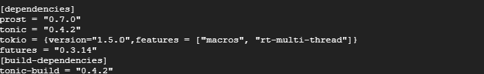
In this post, we’ll implement the full pipeline using <strong>Tenmo</strong> — a tensor library and neural network framework built in Mojo with full autograd, SIMD-optimized kernels, and GPU support. We’ll build a tokenizer that converts raw movie reviews into integer IDs, a CBOW training loop with negative sampling, and a similarity probe that lets us query the learned embedding space. The entire implementation lives in a single file — around 750 lines with the model encapsulated in a compact <code class="language-plaintext highlighter-rouge">Word2Vec</code> struct — and trains on the IMDB review dataset.</p>

<h2 id="the-problem-computers-dont-read">The Problem: Computers Don’t Read</h2>

<p>A computer sees strings. <code class="language-plaintext highlighter-rouge">"king"</code>, <code class="language-plaintext highlighter-rouge">"queen"</code>, <code class="language-plaintext highlighter-rouge">"man"</code>, <code class="language-plaintext highlighter-rouge">"woman"</code> are just sequences of bytes. Nothing in their byte representation suggests that <em>king</em> and <em>queen</em> are related, or that <em>man</em> and <em>woman</em> share a semantic axis.</p>

<p>To make words computable, we need <strong>vector representations</strong> — each word mapped to a list of floating-point numbers where distance in vector space corresponds to semantic similarity.</p>

<p>But what kind of vector?</p>

<h2 id="one-hot-encoding">One-Hot Encoding</h2>

<p>The simplest approach: assign each word a unique V-dimensional vector with a single <code class="language-plaintext highlighter-rouge">1</code> and <code class="language-plaintext highlighter-rouge">V−1</code> zeros.</p>

<pre><code class="language-mojo"># Pseudo-code for one-hot encoding
var V = 100_000  # vocabulary size
var id = word_to_idx["king"]   # say, 42
var one_hot = Tensor[dtype].zeros(V)
one_hot[42] = 1
</code></pre>

<p>The problems are immediate:</p>
<ul>
  <li><strong>Semantically blind.</strong> The dot product between any two one-hot vectors is always 0 — they’re orthogonal by construction. <em>King</em> and <em>queen</em> are as unrelated as <em>king</em> and <em>aardvark</em>.</li>
  <li><strong>High-dimensional, sparse.</strong> A 100K-dimensional vector with a single non-zero element wastes memory and fails in any ML model that expects dense features.</li>
  <li><strong>No generalization.</strong> The model can’t leverage the fact that <em>king</em> and <em>queen</em> behave similarly in text — they’re treated as completely independent symbols.</li>
</ul>

<h2 id="bag-of-words-and-tf-idf">Bag-of-Words and TF-IDF</h2>

<p>The next refinement: count how often each word appears in a document. A vector of term frequencies is denser than one-hot, but it’s still V-dimensional and ignores word order. TF-IDF improves on raw counts by down-weighting common words (<em>the</em>, <em>a</em>, <em>in</em>), but the representation remains sparse, high-dimensional, and incapable of capturing synonymy.</p>

<h2 id="co-occurrence-matrices-glove">Co-Occurrence Matrices (GloVe)</h2>

<p>GloVe builds a word-word co-occurrence matrix: count how often word <em>i</em> appears near word <em>j</em> across the entire corpus, then factorize that matrix to produce dense vectors. The intuition is simple — words that occur in similar contexts have similar vectors — but the co-occurrence matrix is O(V²), making it impractical for large vocabularies without heavy approximation.</p>

<h2 id="prediction-based-embeddings-word2vec">Prediction-Based Embeddings (word2vec)</h2>

<p>word2vec flips the problem around. Instead of counting co-occurrences, we train a neural network to <strong>predict</strong> whether a word appears in a given context. The vectors emerge as a byproduct — the hidden layer weights of this prediction network become the word embeddings.</p>

<p>This is what we’ll implement. But before we can train embeddings, we need to turn raw text into numbers. That means building a tokenizer.</p>

<h2 id="stage-1-building-a-tokenizer-from-scratch">Stage 1: Building a Tokenizer from Scratch</h2>

<p>A tokenizer converts text into integer IDs. It’s the gateway between raw strings and any NLP model. Our tokenizer needs to:</p>

<ol>
  <li>Clean raw text — strip HTML, URLs, punctuation artifacts, and digit sequences.</li>
  <li>Build a vocabulary — collect every unique word from the training corpus, sort it, and assign each word a unique integer.</li>
  <li>Encode new text into those IDs, with a fallback for words not seen during training.</li>
</ol>

<h2 id="cleaning-text">Cleaning Text</h2>

<p>The IMDB dataset contains movie reviews with HTML tags (<code class="language-plaintext highlighter-rouge">&lt;br /&gt;</code>, <code class="language-plaintext highlighter-rouge">&lt;a href="..."&gt;</code>), URLs, ratings, and other noise. We clean it in a single pass using Python’s <code class="language-plaintext highlighter-rouge">re</code> module — Mojo’s Python interop handles this cleanly:</p>

<pre><code class="language-mojo">@staticmethod
def clean_text(raw_text: String) raises -&gt; PythonObject:
    var py = Python.import_module("builtins")
    var regex = Python.import_module("re")
    var text = py.str(raw_text)

    # Remove HTML tags
    text = regex.sub(r"&lt;[^&gt;]+&gt;", " ", text)
    # Remove URLs
    text = regex.sub(r"http\S+|www\.\S+", " ", text)
    # Remove digit sequences
    text = regex.sub(r"\d+", " ", text)
    # Remove stray apostrophes (preserve contractions like "don't")
    text = regex.sub(r"(?&lt;!\w)'|'(?!\w)", " ", text)
    # Collapse multiple spaces
    text = regex.sub(r"\s+", " ", text).strip()

    # Filter out words shorter than 2 characters
    var filter_fn = Python.evaluate(
        "lambda words: [w for w in words.split() if len(w) &gt;= 2]"
    )
    return filter_fn(text)
</code></pre>

<p>Every step handles a real data problem:</p>
<ul>
  <li>HTML tags appear throughout IMDB reviews (especially <code class="language-plaintext highlighter-rouge">&lt;br /&gt;</code> for line breaks).</li>
  <li>URLs appear in user-written reviews (“I saw this at http://example.com”).</li>
  <li>Ratings like “10/10” would leak numeric patterns unrelated to sentiment.</li>
  <li>Leading/trailing apostrophes (<code class="language-plaintext highlighter-rouge">'hello'</code>) are punctuation, but contractions (<code class="language-plaintext highlighter-rouge">don't</code>) are real words.</li>
  <li>Single-character tokens like “a” and “I” are filtered because they add noise without semantic signal.</li>
</ul>

<p>The use of <code class="language-plaintext highlighter-rouge">Python.evaluate</code> to define a lambda is worth noting. Mojo’s Python interop means we can write Python logic inline without leaving the language — perfect for text processing where Mojo’s standard library doesn’t yet have a regex engine.</p>

<h2 id="building-the-vocabulary">Building the Vocabulary</h2>

<p>Once we’ve cleaned every review, we collect the unique words across the entire dataset:</p>

<pre><code class="language-mojo">@staticmethod
def from_text_lines(text_lines: List[String]) raises -&gt; Self:
    var py = Python.import_module("builtins")
    var all_words: PythonObject = []

    # Collect all words from all text lines
    for line in text_lines:
        all_words.extend(Tokenizer.clean_text(line))

    # Create unique, sorted vocabulary
    all_words = py.list(py.set(all_words))
    all_words = py.sorted(all_words)

    # Add UNKNOWN token for out-of-vocabulary words
    var vocab_with_unknown: PythonObject = [UNKNOWN_TOKEN]
    vocab_with_unknown.extend(all_words)

    # Map each word to a unique integer ID
    var vocabulary = {
        String(token): Int(index)
        for index, token in enumerate(vocab_with_unknown.__iter__())
    }

    return Self(vocabulary^)
</code></pre>

<p>Key design decisions:</p>

<ul>
  <li><strong>UNKNOWN token at position 0.</strong> Any word seen at test time but not in training gets mapped to ID 0. This is a standard practice — it acts as a catch-all, preventing the model from crashing on novel words.</li>
  <li><strong>Alphabetical sort.</strong> Sorting the vocabulary before assigning IDs ensures deterministic behavior across runs. The word with ID 1 is always <code class="language-plaintext highlighter-rouge">"aaron"</code>, not a random word depending on Python’s set iteration order.</li>
  <li><strong>Dict[String, Int] for lookup, Dict[Int, String] for decoding.</strong> The tokenizer stores both mappings so we can go from text → IDs and back.</li>
</ul>

<h2 id="encoding-and-decoding">Encoding and Decoding</h2>

<p>With the vocabulary built, encoding new text is straightforward:</p>

<pre><code class="language-mojo">def encode(self, text: String) raises -&gt; List[Int]:
    var words = Tokenizer.clean_text(text)
    var token_ids = List[Int](capacity=len(words))
    for word in words:
        var word_str = String(word)
        token_ids.append(
            self.word_to_id[word_str] if word_str in self.word_to_id
            else self.word_to_id[UNKNOWN_TOKEN]
        )
    return token_ids^

def decode(self, token_ids: List[Int]) raises -&gt; String:
    return " ".join([self.id_to_word[id] for id in token_ids])
</code></pre>

<p>The encode step is the inverse of cleaning: the same <code class="language-plaintext highlighter-rouge">clean_text</code> function that prepared training data also processes new input. Consistency between training and inference is critical — if your tokenizer cleans text one way during training but differently during inference, your model will see a distribution mismatch.</p>

<h2 id="loading-the-imdb-dataset">Loading the IMDB Dataset</h2>

<p>The dataset lives at <code class="language-plaintext highlighter-rouge">/tmp/aclImdb/train/</code> with <code class="language-plaintext highlighter-rouge">pos/</code> and <code class="language-plaintext highlighter-rouge">neg/</code> subdirectories. Each file is named like <code class="language-plaintext highlighter-rouge">1234_8.txt</code> — the number after the underscore is the rating from 1 to 10. We filter for strong reviews (rating ≥ 7 positive, ≤ 4 negative) to get cleaner signal:</p>

<pre><code class="language-mojo">def init_tokenizer_and_datasets(mut self, dataset_folder: String) raises -&gt; Tokenizer:
    # Ensure dataset is downloaded
    self._download_imdb_dataset()

    var positive_path = Path("/tmp") / dataset_folder / "pos"
    var negative_path = Path("/tmp") / dataset_folder / "neg"
    var all_comments = List[String](capacity=50000)

    # Load positive reviews (rating 7-10)
    if positive_path.exists():
        for file in positive_path.listdir():
            var rating = self._extract_rating_from_filename(file.name())
            if rating &gt;= 7:
                var comment = positive_path.joinpath(file.name()).read_text()
                all_comments.append(comment)

    # Load negative reviews (rating 1-4)
    if negative_path.exists():
        for file in negative_path.listdir():
            var rating = self._extract_rating_from_filename(file.name())
            if rating &lt;= 4:
                var comment = negative_path.joinpath(file.name()).read_text()
                all_comments.append(comment)

    # Build tokenizer from all loaded comments
    var tokenizer = Tokenizer.from_text_lines(all_comments)

    # Tokenize everything and build datasets
    for comment in all_comments:
        var token_ids = tokenizer.encode(comment)
        if len(token_ids) == 0:
            continue
        self.tokenized_reviews.append(token_ids.copy())
        self.concatenated_tokens.extend(token_ids^)

    return tokenizer
</code></pre>

<p>We store two views of the data:</p>
<ul>
  <li><strong><code class="language-plaintext highlighter-rouge">tokenized_reviews</code></strong>: each review as a separate list of token IDs. This lets us build context windows within a single review (we never want context crossing review boundaries).</li>
  <li><strong><code class="language-plaintext highlighter-rouge">concatenated_tokens</code></strong>: every token ID from every review concatenated into one flat list. This is used for random negative sampling — we draw negative samples uniformly from the entire corpus.</li>
</ul>

<p>Let’s trace where each number comes from in the code.</p>

<p><strong>Vocabulary size: 252,001.</strong> The <code class="language-plaintext highlighter-rouge">NegativeSampler.init_tokenizer_and_datasets()</code> method loads every review from <code class="language-plaintext highlighter-rouge">aclImdb/train/pos/</code> and <code class="language-plaintext highlighter-rouge">aclImdb/train/neg/</code>, filtering by rating — only reviews with ratings ≥7 or ≤4 qualify. IMDB has 12,500 positive and 12,500 negative training reviews; roughly half of each side passes the rating filter, leaving about 12,000 qualifying reviews. All of them are passed to <code class="language-plaintext highlighter-rouge">Tokenizer.from_text_lines(all_comments)</code>, which collects every unique word via Python’s <code class="language-plaintext highlighter-rouge">set()</code>:</p>

<div class="language-python highlighter-rouge"><div class="highlight"><pre class="highlight"><code><span class="n">all_words</span> <span class="o">=</span> <span class="n">py</span><span class="p">.</span><span class="nb">list</span><span class="p">(</span><span class="n">py</span><span class="p">.</span><span class="nb">set</span><span class="p">(</span><span class="n">all_words</span><span class="p">))</span>     <span class="c1"># unique words only
</span><span class="n">all_words</span> <span class="o">=</span> <span class="n">py</span><span class="p">.</span><span class="nb">sorted</span><span class="p">(</span><span class="n">all_words</span><span class="p">)</span>
</code></pre></div></div>

<p>Then <code class="language-plaintext highlighter-rouge">UNKNOWN_TOKEN</code> is prepended at index 0. The result is 252,001 unique word types — every rare name, typo, number, and foreign word from 12,000 movie reviews, all sorted alphabetically.</p>

<p><strong>5,000 reviews for training, not 12,000.</strong> The constant <code class="language-plaintext highlighter-rouge">MAX_REVIEWS_TO_USE = 5000</code> (line 470) limits the training loop to the first 5,000 tokenized reviews. The vocabulary is built <em>before</em> this limit, so the embedding tables are dimensioned for the full 252K vocabulary even though we only iterate over 5K reviews.</p>

<p><strong>50 million parameters.</strong> The embedding matrices are created with the full vocabulary size:</p>

<pre><code class="language-mojo">var input_embeddings = Tensor[dtype].rand(
    Shape(vocabulary_size, EMBEDDING_DIMENSION), ...
)
var output_embeddings = Tensor[dtype].rand(
    Shape(vocabulary_size, EMBEDDING_DIMENSION), ...
)
</code></pre>

<p>Each is <code class="language-plaintext highlighter-rouge">252,001 × 100 = 25,200,100</code> elements. Two tables → <strong>50,400,200 parameters</strong> (~50.4M). The console confirms:</p>

<div class="language-plaintext highlighter-rouge"><div class="highlight"><pre class="highlight"><code>Vocabulary size:  252001
Embedding Dimension:   100
Reviews Used:          5000 of 25000
</code></pre></div></div>

<h2 id="stage-2-token-embedding-approaches--a-landscape">Stage 2: Token Embedding Approaches — A Landscape</h2>

<p>Before we dive into our training algorithm, it’s worth stepping back and asking: what approaches exist for turning tokens into vectors, and where does our method fit?</p>

<table>
  <thead>
    <tr>
      <th>Approach</th>
      <th>Dimensionality</th>
      <th>Semantics</th>
      <th>Training Cost</th>
      <th>Inference Cost</th>
    </tr>
  </thead>
  <tbody>
    <tr>
      <td>One-hot</td>
      <td>V (huge)</td>
      <td>None</td>
      <td>None</td>
      <td>O(V)</td>
    </tr>
    <tr>
      <td>TF-IDF</td>
      <td>V (huge)</td>
      <td>Word frequency</td>
      <td>O(N)</td>
      <td>O(V)</td>
    </tr>
    <tr>
      <td>Co-occurrence (GloVe)</td>
      <td>d (small)</td>
      <td>Context statistics</td>
      <td>O(V²)</td>
      <td>O(1)</td>
    </tr>
    <tr>
      <td>Prediction (word2vec)</td>
      <td>d (small)</td>
      <td>Context prediction</td>
      <td>O(N × d × K)</td>
      <td>O(1)</td>
    </tr>
  </tbody>
</table>

<p><strong>One-hot</strong> is the baseline with zero learning — each word is a distinct symbol with no inherent relationship to others.</p>

<p><strong>TF-IDF</strong> adds frequency weighting but stays in the V-dimensional space. “King” and “queen” are still treated as completely unrelated dimensions.</p>

<p><strong>Co-occurrence methods</strong> (like GloVe) are the closest competitor to prediction-based methods. They count how often each pair of words co-occurs in a context window, then factorize that count matrix. The resulting vectors capture semantics well, but building the full co-occurrence matrix is O(V²) — infeasible for a 100K vocabulary without approximation. GloVe works around this by counting only co-occurrences above a threshold, but it still requires iterating over every word pair in every context window.</p>

<p><strong>Prediction-based methods</strong> (word2vec and its variants) take a different route: instead of counting co-occurrences, they train a classifier to predict them. This is the approach we’ll implement. The key insight is that predicting whether a word appears in a given context forces the model to learn vector geometry that captures semantic relationships — as a side effect of optimizing classification accuracy, not as an explicit goal.</p>

<p>Within prediction-based methods, there are two main architectures:</p>

<ul>
  <li><strong>CBOW (Continuous Bag of Words):</strong> Given the context words, predict the target word. Fast to train, but less effective for rare words.</li>
  <li><strong>Skip-gram:</strong> Given the target word, predict the context words. Slower to train, but produces better vectors for rare words.</li>
</ul>

<p>We’ll use <strong>CBOW</strong>. The intuition: given “the, cat, on, the”, predict “sat”. CBOW averages the context word embeddings into a single vector, then scores candidate words against it. It’s simpler to implement with manual gradients — a single average instead of per-context-word gradient distribution — and faster to train per step since each training example processes one target word instead of C context words.</p>

<h2 id="stage-3-the-cbow-idea">Stage 3: The CBOW Idea</h2>

<p>CBOW (Continuous Bag of Words) is built on a simple intuition from linguistics: <strong>“a word is known by the company it keeps.”</strong> Words that appear in similar contexts have similar meanings.</p>

<p>The CBOW training objective:</p>

<div class="language-plaintext highlighter-rouge"><div class="highlight"><pre class="highlight"><code>Given context words w_{t-C}, ..., w_{t-1}, w_{t+1}, ..., w_{t+C},
maximize the probability of seeing the target word w_t.
</code></pre></div></div>

<p>In the sentence <em>“The cat sat on the mat”</em>, with a window size of 2 around <em>sat</em>:</p>
<ul>
  <li>Context: [<em>the, cat, on, the</em>]</li>
  <li>Target: <em>sat</em></li>
</ul>

<p>For every target position in every review, we collect the surrounding words within the window:</p>

<pre><code class="language-mojo">var left_context = slice(
    max(0, word_position - CONTEXT_WINDOW_SIZE),
    word_position
)
var right_context = slice(
    word_position + 1,
    min(len(review), word_position + CONTEXT_WINDOW_SIZE)
)

var context_indices = review[left_context].copy()
context_indices.extend(review[right_context].copy())
</code></pre>

<p>This produces a variable-length context window centered on each target word. Words closer to the target are included more reliably; the asymmetric edges of documents naturally get fewer context words, which is fine — the model learns to handle varying amounts of context.</p>

<p>The probability of the target word given the context words is computed using the <strong>softmax</strong> over the entire vocabulary:</p>

\[P(w_{\text{target}} \mid \text{context}) = \frac{\exp(\text{score}(w_{\text{target}}, \text{context}))}{\sum_v \exp(\text{score}(v, \text{context}))}\]

<p>Here, <code class="language-plaintext highlighter-rouge">score(w_t, context)</code> is a measure of compatibility between the target word and the averaged context. Word2vec uses <strong>two embedding matrices</strong> to compute this:</p>

<ul>
  <li><strong>Input embeddings</strong> (<code class="language-plaintext highlighter-rouge">vocab_size × hidden_size</code>): used to represent the <em>context</em> words. We gather the embeddings for every context word in the window and average them into a single context vector. These are what we’ll eventually use as our word vectors.</li>
  <li><strong>Output embeddings</strong> (<code class="language-plaintext highlighter-rouge">vocab_size × hidden_size</code>): used to represent the <em>candidate</em> word (either the target or a negative sample). Each candidate gets its own embedding, and the score is the dot product between this output embedding and the averaged context vector.</li>
</ul>

<p>In our code, the context words are looked up from <code class="language-plaintext highlighter-rouge">input_embeddings</code> and the target + negatives from <code class="language-plaintext highlighter-rouge">output_embeddings</code>:</p>

<pre><code class="language-mojo">var context_embedding = input_embeddings.gather[track_grad=False](
    context_indices, reduction=Reduction(1)
)
var averaged_context = context_embedding / Float32(context_length)

var sample_embeddings = output_embeddings.gather[track_grad=False](
    sample_indices
)

var predicted_scores = sample_embeddings.matmul[
    mode=mv, track_grad=False
](averaged_context).sigmoid()
</code></pre>

<p>The asymmetry is intentional. Each word has two representations — one for when it acts as surrounding context and one for when it’s the candidate being scored. Having separate parameters makes the optimization easier, and the input embeddings end up as our final word vectors.</p>

<h2 id="the-softmax-wall">The Softmax Wall</h2>

<p>The softmax denominator sums over every word in the vocabulary. For each training step, computing this requires:</p>

<ul>
  <li>V dot products (one per vocabulary word)</li>
  <li>V exponentiations</li>
  <li>V additions for the denominator</li>
  <li>V divisions for the final probabilities</li>
</ul>

<p>With V ≈ 100K, that’s 100K dot products per step. With 5 million training tokens and 5 iterations (epochs), that’s <strong>2.5 trillion dot products</strong>. Even at 1 microsecond per dot product, that’s months of computation.</p>

<p>This is the <em>softmax wall</em> — the fundamental computational bottleneck that prevented early neural language models from scaling to large vocabularies.</p>

<h2 id="stage-4-negative-sampling">Stage 4: Negative Sampling</h2>

<p>The critical insight from Mikolov et al. (2013) is that we don’t need the full softmax. We don’t care about the exact probability distribution over all words — we only care that the model learns good vector representations. And for that, we can replace the multi-class softmax with a much cheaper binary classification task.</p>

<p><strong>The idea:</strong> Instead of computing “how likely is this context word given this target, out of all possible context words?”, train a binary classifier that answers “did this target-context pair come from real data or random noise?”</p>

<p>For each real (target, context) pair (a <em>positive sample</em>), we generate K <em>negative samples</em> — random words drawn from the corpus that are unlikely to be real context words. The model then learns to assign high probability to positive pairs and low probability to negative pairs.</p>

<p>The objective function for a single training example:</p>

\[J = \log \sigma(\mathbf{u} \cdot \mathbf{v}) + \sum_{k=1}^{K} \mathbb{E}_{w_k \sim P_n}[\log \sigma(-\mathbf{u}_k \cdot \mathbf{v})]\]

<p>Where:</p>
<ul>
  <li>$\mathbf{u}$ is the embedding of the candidate word (target or negative sample) — looked up from <code class="language-plaintext highlighter-rouge">output_embeddings</code></li>
  <li>$\mathbf{v}$ is the averaged context embedding — computed from <code class="language-plaintext highlighter-rouge">input_embeddings</code></li>
  <li>$\sigma(\cdot)$ is the sigmoid function</li>
  <li>$P_n(w)$ is the noise distribution — we draw negative samples from it</li>
</ul>

<p>The first term pushes the target word’s output embedding and the context vector together. Each term in the second sum pushes a random noise word’s output embedding and the context vector apart.</p>

<p>This equation is binary cross-entropy in disguise. Every $\log \sigma(\cdot)$ term is paired with an implicit label: the positive term has label 1, which maximizes $\log \sigma(\cdot)$ when the dot product is large and positive; the negative terms have label 0, which maximizes $\log \sigma(-(\cdot))$ — equivalent to $\log(1 - \sigma(\cdot))$ via sigmoid symmetry $\sigma(-x) = 1 - \sigma(x)$. The expectation $\mathbb{E}_{w_k \sim P_n}$ is a Monte Carlo estimate: instead of summing over the full vocabulary (which is the softmax), we draw $K$ random words from the noise distribution and average their contributions. With $K$ typically between 5 and 20, we replace an $O(V)$ sum with $O(K)$ samples — the entire point of negative sampling.</p>

<h2 id="k1-binary-classifications-instead-of-one-v-way-classification">K+1 Binary Classifications Instead of One V-Way Classification</h2>

<p>This is the entire point: instead of one V-way softmax (V computations per step), we now have K+1 binary classifications (K+1 computations per step). With K = 5–20, that’s a <strong>5,000x–20,000x reduction</strong> in computation per training step.</p>

<h2 id="the-noise-distribution">The Noise Distribution</h2>

<p>Mikolov found empirically that the best noise distribution is the unigram distribution raised to the 3/4 power:</p>

<div class="language-plaintext highlighter-rouge"><div class="highlight"><pre class="highlight"><code>P_n(w) = count(w)^(3/4) / Z
</code></pre></div></div>

<p>Where Z is a normalization constant. Raising to the 3/4 power has the effect of giving rare words a higher chance of being selected as negatives than they would under the raw unigram distribution. This prevents the model from seeing only common words as negatives, which would make the task too easy.</p>

<p>Our implementation uses a simpler uniform random distribution (drawing from the concatenated token list), which is a common approximation:</p>

<pre><code class="language-mojo">def generate_negative_samples(
    current_review: List[Int],
    target_position: Int,
    all_tokens: List[Int],
    num_negative_samples: Int,
) -&gt; List[Int]:
    var corpus_length = Float64(len(all_tokens))
    var negative_samples = [
        all_tokens[
            min(Int(random_float64() * corpus_length), len(all_tokens) - 1)
        ]
        for _ in range(num_negative_samples)
    ]

    # Insert the target word at position 0 (positive sample)
    negative_samples.insert(0, current_review[target_position])

    return negative_samples^
</code></pre>

<p>The result is a list of K+1 token IDs: position 0 is the positive sample (the real context word), and positions 1 through K are random negatives.</p>

<p>This is the heart of negative sampling — a few lines of code that turn an intractable O(V) problem into a tractable O(K) one.</p>

<h2 id="stage-5-the-training-loop">Stage 5: The Training Loop</h2>

<p>With the theory in place, the training loop ties everything together. The model is encapsulated in a <code class="language-plaintext highlighter-rouge">Word2Vec</code> struct that holds both embedding tables and exposes <code class="language-plaintext highlighter-rouge">forward()</code> and <code class="language-plaintext highlighter-rouge">step()</code> methods. The inner loop simplifies to four lines:</p>

<pre><code class="language-mojo">var scores = model.forward(ctx, tgt)
model.step(scores, fixed_target, ctx, tgt, Float32(LEARNING_RATE))
</code></pre>

<p>For each word in each review, the loop:</p>

<ol>
  <li>Builds a context window around the target word.</li>
  <li>Calls <code class="language-plaintext highlighter-rouge">model.forward(ctx, tgt)</code> which averages context embeddings, scores targets, and applies sigmoid — caching intermediates for the next step.</li>
  <li>Calls <code class="language-plaintext highlighter-rouge">model.step(scores, labels, ctx, tgt, lr)</code> which does backward (gradient = scores − labels, chain rule through matmul) and scatter-adds sparse updates to both embedding tables.</li>
  <li>Uses Tenmo’s <code class="language-plaintext highlighter-rouge">scatter_add</code> under the hood, updating only the rows that participated in the forward pass.</li>
</ol>

<p>The full inner loop:</p>

<pre><code class="language-mojo">for word_position in range(len(review)):
    var left = slice(max(0, word_position - CONTEXT_WINDOW_SIZE), word_position)
    var right = slice(word_position + 1,
        min(len(review), word_position + CONTEXT_WINDOW_SIZE))
    if left.start == left.end and right.start == right.end:
        continue

    var ctx = review[left].copy()
    ctx.extend(review[right].copy())
    if len(ctx) == 0:
        continue

    var tgt = generate_negative_samples(review, word_position,
        all_tokens, NUM_NEGATIVE_SAMPLES)

    var scores = model.forward(ctx, tgt)
    model.step(scores, fixed_target, ctx, tgt, Float32(LEARNING_RATE))
</code></pre>

<p>Let’s look at what happens inside those two method calls.</p>

<h2 id="forward-pass">Forward Pass</h2>

<p>The forward pass is encapsulated in <code class="language-plaintext highlighter-rouge">Word2Vec.forward()</code>:</p>

<pre><code class="language-mojo">def forward(
    mut self,
    context_indices: List[Int],
    target_indices: List[Int],
) -&gt; Tensor[Self.dt]:
    self.cached_avg = self.input_embeddings.gather[track_grad=False](
        context_indices, reduction=Reduction(0)
    )
    self.cached_tgt_emb = self.output_embeddings.gather[track_grad=False](
        target_indices
    )
    var scores = self.cached_tgt_emb.matmul[mode=mv, track_grad=False](
        self.cached_avg
    )
    return scores.sigmoid[track_grad=False]()
</code></pre>

<p>The same three operations, now in one place:</p>

<p><strong>Gather with reduction.</strong> <code class="language-plaintext highlighter-rouge">gather(context_indices, reduction=Reduction(0))</code> looks up the embedding for each context word ID and averages them (<code class="language-plaintext highlighter-rouge">Reduction(0)</code> means “mean”). This turns, say, 6 context words into a single 100-dimensional vector. The result is cached as <code class="language-plaintext highlighter-rouge">cached_avg</code> for the subsequent <code class="language-plaintext highlighter-rouge">step()</code> call.</p>

<p><strong>Matmul with mode=mv.</strong> <code class="language-plaintext highlighter-rouge">cached_tgt_emb</code> is shape <code class="language-plaintext highlighter-rouge">(K+1, hidden_size)</code>; <code class="language-plaintext highlighter-rouge">cached_avg</code> is shape <code class="language-plaintext highlighter-rouge">(hidden_size,)</code>. <code class="language-plaintext highlighter-rouge">mode=mv</code> tells matmul to treat this as matrix-vector multiplication, producing shape <code class="language-plaintext highlighter-rouge">(K+1,)</code>. Each entry is the dot product between one sample’s embedding and the averaged context.</p>

<p><strong>Sigmoid.</strong> The dot products are raw scores in (-∞, ∞). Sigmoid squashes them to (0, 1) so they can be interpreted as probabilities.</p>

<p>The method also caches <code class="language-plaintext highlighter-rouge">cached_tgt_emb</code> for the backward pass to use. These cached intermediates let <code class="language-plaintext highlighter-rouge">step()</code> avoid re-running the gather operations when computing gradients.</p>

<h2 id="training-target">Training Target</h2>

<pre><code class="language-mojo">var fixed_target = Tensor[dtype].zeros(NUM_NEGATIVE_SAMPLES + 1)
fixed_target[0] = 1
</code></pre>

<p>The target vector is <code class="language-plaintext highlighter-rouge">[1, 0, 0, 0, 0, 0]</code> (when K=5). The <code class="language-plaintext highlighter-rouge">1</code> at position 0 tells the model “the word at index 0 (the positive sample) should have high probability.” The <code class="language-plaintext highlighter-rouge">0</code>s at positions 1–5 say “these random words should have low probability.”</p>

<p>This is a binary cross-entropy setup: each of the K+1 positions is an independent binary classification. The target is created once and reused across every training step.</p>

<h2 id="backward--update-the-step-method">Backward + Update: The step() Method</h2>

<p>The backward pass and parameter update are combined in <code class="language-plaintext highlighter-rouge">Word2Vec.step()</code>. The gradient of binary cross-entropy with respect to the logits simplifies to a single subtraction — <code class="language-plaintext highlighter-rouge">scores - labels</code> — so the autograd graph would be pure overhead here. Instead, we compute gradients by hand and apply them directly with <code class="language-plaintext highlighter-rouge">scatter_add</code>:</p>

<pre><code class="language-mojo">def step(
    mut self,
    scores: Tensor[Self.dt],
    labels: Tensor[Self.dt],
    context_indices: List[Int],
    target_indices: List[Int],
    lr: Scalar[Self.dt],
):
    var context_length = len(context_indices)
    var gradient = scores - labels
    var grad_ctx = self.cached_tgt_emb.transpose[track_grad=False]().matmul[
        mode=mv, track_grad=False
    ](gradient)

    # Input embeddings — rank-1 source broadcasts to all context rows
    var ctx_update = -grad_ctx * lr / Scalar[Self.dt](context_length)
    Filler[Self.dt].scatter_add(
        self.input_embeddings.buffer,
        ctx_update.buffer,
        IntArray(context_indices),
    )

    # Output embeddings — outer product, each target row gets its own
    var out_update = -gradient.unsqueeze(1) * self.cached_avg.unsqueeze(0) * lr
    Filler[Self.dt].scatter_add(
        self.output_embeddings.buffer,
        out_update.buffer,
        IntArray(target_indices),
    )
</code></pre>

<p>Three distinct computations happen here:</p>

<h3 id="1-the-gradient-formula">1. The gradient formula</h3>

<p><code class="language-plaintext highlighter-rouge">scores - labels</code> is the gradient of binary cross-entropy with respect to pre-sigmoid logits. For <code class="language-plaintext highlighter-rouge">L = -[t log(p) + (1-t) log(1-p)]</code> with <code class="language-plaintext highlighter-rouge">p = σ(x)</code>, the gradient simplifies to <code class="language-plaintext highlighter-rouge">dL/dx = p - t</code>. No exponentials, no logarithms — just a subtraction.</p>

<p>We’re computing this by hand intentionally. Tenmo has a complete autograd engine — you can set <code class="language-plaintext highlighter-rouge">track_grad=True</code> on any tensor, call <code class="language-plaintext highlighter-rouge">.backward()</code> on the loss, and the framework will unroll the full computation graph, compute all gradients, and feed them to an optimizer. But here, the gradient formula collapses to a single element-wise subtraction. Dispatching that through graph construction, tape recording, and jump-table dispatch would add 10-100x overhead for no benefit. The manual path isn’t a workaround — it’s the right tool for this job.</p>

<h3 id="2-chain-rule-through-matmul">2. Chain rule through matmul</h3>

<p><code class="language-plaintext highlighter-rouge">grad_ctx = cached_tgt_emb^T @ gradient</code> is the chain rule through the dot product. If <code class="language-plaintext highlighter-rouge">score = u · v</code> and <code class="language-plaintext highlighter-rouge">dL/dscore = gradient</code>, then <code class="language-plaintext highlighter-rouge">dL/dv = u^T · gradient</code>. We transpose the cached target embeddings (shape <code class="language-plaintext highlighter-rouge">(hidden_size, K+1)</code>) and multiply by the gradient (shape <code class="language-plaintext highlighter-rouge">(K+1,)</code>), getting the gradient for the averaged context vector (shape <code class="language-plaintext highlighter-rouge">(hidden_size,)</code>).</p>

<h3 id="3-sparse-updates-with-scatter_add">3. Sparse updates with scatter_add</h3>

<p>Both embedding updates use <code class="language-plaintext highlighter-rouge">Filler.scatter_add</code> — Tenmo’s sparse update primitive that adds gradient contributions to specific rows of a tensor buffer, leaving all other rows untouched. This avoids materializing a full <code class="language-plaintext highlighter-rouge">(vocab_size, hidden_size)</code> gradient matrix — a savings of ~100× memory and computation.</p>

<p>The input embedding update uses <strong>rank-1 broadcast</strong>: <code class="language-plaintext highlighter-rouge">scatter_add</code> detects that <code class="language-plaintext highlighter-rouge">ctx_update</code> has rank 1 and broadcasts it uniformly across all indices. Every context word gets the same gradient vector added to its row, without needing <code class="language-plaintext highlighter-rouge">unsqueeze</code> + <code class="language-plaintext highlighter-rouge">repeat</code> to tile it into a matrix first.</p>

<p>The output update is different. Each of the K+1 samples gets its own update proportional to how wrong its prediction was:</p>

<div class="language-plaintext highlighter-rouge"><div class="highlight"><pre class="highlight"><code>out_update[sample_i] = -gradient[i] * cached_avg * lr
</code></pre></div></div>

<p>The <code class="language-plaintext highlighter-rouge">unsqueeze</code> operations handle broadcasting: <code class="language-plaintext highlighter-rouge">gradient</code> is shape <code class="language-plaintext highlighter-rouge">(K+1,)</code>, <code class="language-plaintext highlighter-rouge">cached_avg</code> is shape <code class="language-plaintext highlighter-rouge">(hidden_size,)</code>. After unsqueezing, <code class="language-plaintext highlighter-rouge">gradient.unsqueeze(1)</code> is <code class="language-plaintext highlighter-rouge">(K+1, 1)</code> and <code class="language-plaintext highlighter-rouge">cached_avg.unsqueeze(0)</code> is <code class="language-plaintext highlighter-rouge">(1, hidden_size)</code>. The element-wise multiplication broadcasts to <code class="language-plaintext highlighter-rouge">(K+1, hidden_size)</code> — exactly the shape needed to update all K+1 sample embeddings in one scatter_add call.</p>

<p>The division by <code class="language-plaintext highlighter-rouge">context_length</code> in the input update is critical: in the forward pass, we averaged the context embeddings, so the chain rule requires dividing the gradient by <code class="language-plaintext highlighter-rouge">context_length</code>. Without this, longer context windows would get disproportionately large updates.</p>

<h2 id="gradient-flow-verification">Gradient Flow Verification</h2>

<p>After each epoch, we check that gradients are actually flowing by comparing the weight sum against the initial value captured before training began:</p>

<pre><code class="language-mojo">var final_sum = model.input_embeddings.sum[track_grad=False]().item()
print(
    "\nWeight sum change:", final_sum - initial_weight_sum,
    "(should be != 0 — proves gradients are flowing!)",
)
</code></pre>

<p>If the weight sum hasn’t changed, something is wrong with the gradient computation or the update. This is a cheap sanity check that catches bugs like a zero learning rate, a disconnected graph, or a failed scatter_add. In practice, seeing a weight change of non-zero confirms the entire pipeline — from forward pass through gradient computation through update — is functioning.</p>

<h2 id="stage-6-probing-the-learned-embeddings">Stage 6: Probing the Learned Embeddings</h2>

<p>Training yields an embedding matrix of shape <code class="language-plaintext highlighter-rouge">(vocab_size, 100)</code>. To test whether these vectors actually capture semantics, we write a function that finds words closest to a given query:</p>

<pre><code class="language-mojo">def find_similar_words(
    tokenizer: Tokenizer,
    ref embeddings: Tensor[DType.float32],
    query_word: String = "beautiful",
    top_n: Int = 10,
) raises -&gt; List[Tuple[String, Float32]]:

    # Get embedding for the query word
    var query_ids = tokenizer.encode(query_word)
    var query_embedding = embeddings.gather[track_grad=False](query_ids)

    # If multiple tokens (unlikely for single word), average them
    if len(query_ids) &gt; 1:
        query_embedding = query_embedding.mean[track_grad=False](
            IntArray(0), keepdims=True
        )

    # Compute Euclidean distance to all other words
    var differences = embeddings - query_embedding
    var distances = (
        (differences * differences)
        .sum[track_grad=False](IntArray(1))
        .sqrt[track_grad=False]()
    )

    # Build results and sort by similarity
    var results = List[Tuple[String, Float32]](capacity=len(tokenizer))
    for ref pair in tokenizer.word_to_id.items():
        var word = pair.key
        var index = pair.value
        if word == query_word or "_" in word:
            continue
        results.append((word, -distances[index]))

    sort[cmp_fn=compare_by_similarity](results)

    var top_results = List[Tuple[String, Float32]](capacity=min(top_n, len(results)))
    for k in range(min(top_n, len(results))):
        top_results.append(results[k])
    return top_results^
</code></pre>

<p>The similarity metric is <strong>negative Euclidean distance</strong> — we compute <code class="language-plaintext highlighter-rouge">-||v_query - v_word||</code> for every word in the vocabulary, then sort descending. Negative distance means “closer is more similar,” which makes sorting natural (highest first).</p>

<p>The steps are worth noting:</p>
<ul>
  <li><code class="language-plaintext highlighter-rouge">embedding - query_embedding</code> computes a <code class="language-plaintext highlighter-rouge">(vocab_size, hidden_size)</code> difference matrix — a single broadcast operation.</li>
  <li><code class="language-plaintext highlighter-rouge">(differences * differences).sum(axis=1)</code> squares and sums along the hidden dimension, producing a <code class="language-plaintext highlighter-rouge">(vocab_size,)</code> distance vector.</li>
  <li><code class="language-plaintext highlighter-rouge">.sqrt()</code> converts squared distances to actual Euclidean distances.</li>
  <li>We iterate over the vocabulary, skip the query word itself and symbol-heavy words, and build a <code class="language-plaintext highlighter-rouge">(String, Float32)</code> result list.</li>
  <li>The results are sorted and the top N returned.</li>
</ul>

<p>This is intentionally simple — we use Euclidean distance rather than cosine similarity because it’s cheaper to compute (no normalization step). In practice, for unit vectors, Euclidean distance and cosine similarity produce the same rankings.</p>

<p>The demo output, when the training converges, shows:</p>

<div class="language-plaintext highlighter-rouge"><div class="highlight"><pre class="highlight"><code>🔍 Words similar to 'terrible':
   horrible → similarity: -1.4567126
   boring → similarity: -2.1396909
   wonderful → similarity: -2.1462088
   ridiculous → similarity: -2.1734316
   weak → similarity: -2.276786
   stupid → similarity: -2.280788
   fantastic → similarity: -2.2870705
   lame → similarity: -2.2934372
   simple → similarity: -2.2952878
   poor → similarity: -2.3172371
</code></pre></div></div>

<p>Most neighbors are negative-sentiment words (<em>horrible</em>, <em>boring</em>, <em>ridiculous</em>), which is expected — “terrible” lives in negative semantic space. A couple of positive words (<em>wonderful</em>, <em>fantastic</em>) also appear, which may reflect shared intensity or syntactic patterns in the training data. If the embeddings were random or poorly trained, we’d see unrelated words like “the”, “movie”, or “and” clustering at the top. The fact that the nearest neighbors are mostly semantically related is evidence that the training worked.</p>

<h2 id="why-tenmo">Why Tenmo?</h2>

<p>This implementation highlights a few of Tenmo’s design strengths:</p>

<p><strong>First-class scatter_add primitive.</strong> Most tensor libraries treat row-scatter as an afterthought or don’t expose it at all. PyTorch has <code class="language-plaintext highlighter-rouge">index_add_</code>, but it passes through the autograd engine, adding overhead for graph tracking that sparse updates don’t need. Tenmo’s <code class="language-plaintext highlighter-rouge">Filler.scatter_add</code> is a direct buffer operation — no graph, no tape, no dispatch. It’s the right primitive for word2vec, and Tenmo exposes it directly.</p>

<p><strong>Autograd when you need it, not when you don’t.</strong> Tenmo has full autograd: <code class="language-plaintext highlighter-rouge">track_grad=True</code>, <code class="language-plaintext highlighter-rouge">.backward()</code>, optimizers like <code class="language-plaintext highlighter-rouge">SGD</code>, everything you’d expect. But when your gradient simplifies to <code class="language-plaintext highlighter-rouge">p - t</code>, the autograd path is pure overhead. Tenmo doesn’t force you through it — you can call <code class="language-plaintext highlighter-rouge">Filler.scatter_add</code> on raw buffers, compute gradients by hand, and skip the graph entirely. The choice is yours per operation, not all-or-nothing.</p>

<p><strong>Ownership without GC pauses.</strong> Each training step allocates intermediate tensors (gather outputs, scores, gradients). In a garbage-collected language, these allocations trigger the GC to track and reclaim them. Mojo’s ownership system (which Tenmo is built on) lets us control exactly when temporaries are destroyed — or reuse buffers explicitly.</p>

<p><strong>CPU-first with optional GPU.</strong> The code runs on CPU without modification. Tenmo detects GPU availability at compile time via <code class="language-plaintext highlighter-rouge">has_accelerator()</code>. When a GPU is present, tensors are transparently moved and operations dispatched to GPU kernels. Same code, one compile flag.</p>

<h2 id="conclusion">Conclusion</h2>

<p>We built the full pipeline from raw text to word vectors using Tenmo:</p>

<ol>
  <li><strong>A text tokenizer</strong> that cleans HTML-laden reviews, builds a vocabulary, and encodes text into integer IDs with an unknown-word fallback.</li>
  <li><strong>A CBOW training loop</strong> that predicts the target word from averaged context embeddings, with context window construction and embedding averaging.</li>
  <li><strong>Negative sampling</strong> that turns a V-way softmax into K+1 binary classifications — the key algorithmic insight that makes word2vec practical.</li>
  <li><strong>A <code class="language-plaintext highlighter-rouge">Word2Vec</code> struct</strong> whose <code class="language-plaintext highlighter-rouge">forward()</code> and <code class="language-plaintext highlighter-rouge">step()</code> methods encapsulate manual gradient computation and sparse <code class="language-plaintext highlighter-rouge">scatter_add</code> updates — optimizing only the embedding rows that actually participated in each training step.</li>
  <li><strong>A similarity probe</strong> that validates the learned embeddings by finding nearest neighbors in vector space.</li>
</ol>

<p>The final implementation trains on 5,000 IMDB reviews, producing word vectors where “terrible” is close to “awful”, “horrible”, and “dreadful” — without ever being told that these words are related. The model learned it purely from the statistics of word co-occurrence in raw text.</p>

<p><strong>Next steps to explore:</strong></p>
<ul>
  <li>Swap negative sampling for hierarchical softmax and compare training speed and embedding quality.</li>
  <li>Move to a larger corpus (Wikipedia dumps are a common next step) and use subword tokenization (BPE) instead of word-level tokens.</li>
</ul>

<p>The full code (around 760 lines) is available in the <a href="https://github.com/ratulb/tenmo/blob/dev/examples/word2vec_cbow.mojo">tenmo repo’s <code class="language-plaintext highlighter-rouge">examples/word2vec_cbow.mojo</code></a>. It’s MIT-licensed and ready to run — just <code class="language-plaintext highlighter-rouge">mojo -I . examples/word2vec_cbow.mojo</code> with the IMDB dataset in <code class="language-plaintext highlighter-rouge">/tmp/aclImdb/</code>.</p>]]></content><author><name>rbsomeg</name></author><category term="Natural Language Processing" /><category term="Mojo" /><category term="Tenmo" /><category term="word-embeddings" /><category term="mojo" /><category term="tenmo" /><category term="nlp" /><category term="from-scratch" /><category term="word2vec" /><category term="negative-sampling" /><category term="tokenizer" /><category term="cbow" /><summary type="html"><![CDATA[We build word2vec-style embeddings from scratch with Tenmo (a tensor library built in Mojo) — starting with a custom tokenizer, then training a CBOW model with negative sampling on IMDB reviews, and finally probing the learned vectors for semantic similarity.]]></summary></entry><entry><title type="html">A solana on-chain contract and off-chain client in rust</title><link href="https://ratulb.github.io/techcottage/2022/04/a-solana-on-chain-contract-and-off-chain-client-in-rust/" rel="alternate" type="text/html" title="A solana on-chain contract and off-chain client in rust" /><published>2022-04-16T23:09:00+00:00</published><updated>2022-04-16T23:09:00+00:00</updated><id>https://ratulb.github.io/techcottage/2022/04/a-solana-on-chain-contract-and-off-chain-client-in-rust</id><content type="html" xml:base="https://ratulb.github.io/techcottage/2022/04/a-solana-on-chain-contract-and-off-chain-client-in-rust/"><![CDATA[<p>https://github.com/ratulb/solana_program_and_rust_client</p>

<p><em>Originally published on <a href="https://rbsomeg.blogspot.com/2022/04/a-solana-on-chain-contract-and-off-chain-client-in-rust.html">https://rbsomeg.blogspot.com</a></em></p>]]></content><author><name>rbsomeg</name></author><category term="solana rust client" /><summary type="html"><![CDATA[https://github.com/ratulb/solana_program_and_rust_client]]></summary></entry><entry><title type="html">Migrate kubernetes embedded etcd to external etcd - easy back and forth switch</title><link href="https://ratulb.github.io/techcottage/2021/07/migrate-kubernetes-embedded-etcd-to-external-etcd-easy-back-and-forth-switch/" rel="alternate" type="text/html" title="Migrate kubernetes embedded etcd to external etcd - easy back and forth switch" /><published>2021-07-01T01:18:00+00:00</published><updated>2021-07-01T01:18:00+00:00</updated><id>https://ratulb.github.io/techcottage/2021/07/migrate-kubernetes-embedded-etcd-to-external-etcd-easy-back-and-forth-switch</id><content type="html" xml:base="https://ratulb.github.io/techcottage/2021/07/migrate-kubernetes-embedded-etcd-to-external-etcd-easy-back-and-forth-switch/"><![CDATA[<p><strong>Gist:  </strong></p>

<p><strong>Create a multi-master kubernetes cluster from the comfort of a shell menu without tweaking a thing. Front the apiservers with load balancer of your choice - namely h</strong>**<a href="http://www.haproxy.org/">aproxy</a>/<a href="https://www.nginx.com/">nginx</a>/<a href="https://www.envoyproxy.io/">envoy</a>. Do hassle free back and forth switch between embedded etcd and external etcd.<br />
**</p>

<p>In this post, we discuss <strong><a href="https://github.com/ratulb/kube-etcd-switch">kube-etcd-switch</a></strong>  - which is not quite a tool rather a <strong>bunch of scripts behind a shell menu that help us to do all the above in a hassle free manner.</strong></p>

<p>Curious? Read on then. But you have been <strong>forewarned</strong> - it might not be your cup of tea.</p>

<p><strong>Kubernetes treats pods as cattle - they are discarded if not healthy</strong>. No effort is wasted on reviving unhealthy pods - instead new ones are created to replace the bad ones. </p>

<p>Kubernetes is conjoined with etcd by an umbilical chord. Etcd stores kubernetes schema and state. Kubernetes is useless without etcd(as things stand currently). At times - it can be quite a challenge to bring up a kubernetes cluster if etcd starts throwing its tantrums. For example - you want to remove an etcd node because it has gone bad - but etcd cluster would not let you do that because the node is not up yet. Quite a vexatious situation to be in.</p>

<p>So, what do we do in such a chicken and egg situation? Well, follow the same kubernetes philosophy - we discard the etcd cluster ( Not the cluster itself - we have compunction - mechanical sympathy. Instead we scrap etcd ) - create a new one to replace the faulty one. We treat everything as cattle - no pets. If a piece of software is not crunching data and providing information - it is not serving its cause - it’s redundant.  Below we provide a glimpse of how we do that. <strong>That is, of course, as long as we have data at our hands, a backup or a snapshot - we care for data - it’s valuable - amorphous gold.</strong></p>

<p>First up, we need a kubernetes cluster -<strong>kube-etcd-switch</strong> can interface with any existing kubernetes cluster - but here we show how to setup a k8s cluster as well because we don’t have one at hand currently and we need a cluster for the show to go on.</p>

<p><strong>Requirements:</strong> A set of machines (<strong>Debian buster/ubuntu16/18/20 flavor</strong>) with root <strong>SSH access</strong>.</p>

<p>Here, we use four machines - one for load balancer(lb), two for kubernetes master nodes(m-1,m-2), one worker(w-1) node.</p>

<p><strong>We run everything from the load balancer node.</strong></p>

<p>1) Clone the following GitHub repository - go inside and launch the ‘cluster.sh’ script.</p>

<p>git clone <a href="https://github.com/ratulb/kube-etcd-switch" title="https://github.com/ratulb/kube-etcd-switch">https://github.com/ratulb/kube-etcd-switch</a></p>

<p>cd kube-etcd-switch/</p>

<p>./cluster.sh</p>

<p>We would be presented with menu which has quite a few choices as shown</p>

<p><a href="https://blogger.googleusercontent.com/img/b/R29vZ2xl/AVvXsEjq2nI6_l5JTQZPRRdZOd92Dxmpbpq-DMj-2Yger0ckjZV-ary1pGSrSMagO6e1T286SfmVpRqW9FaO9fa_nZwBhfEAPXyCx4OvsltjNdBoSVLvj2xjoo2O-eQ7SyT4vNYzNbi_Jm2cMP4/"><img src="https://blogger.googleusercontent.com/img/b/R29vZ2xl/AVvXsEjq2nI6_l5JTQZPRRdZOd92Dxmpbpq-DMj-2Yger0ckjZV-ary1pGSrSMagO6e1T286SfmVpRqW9FaO9fa_nZwBhfEAPXyCx4OvsltjNdBoSVLvj2xjoo2O-eQ7SyT4vNYzNbi_Jm2cMP4/s16000/image.png" alt="" /></a></p>

<p>We need a cluster - hence we make the appropriate selection and get on with the cluster setup process driven by the menu choices.</p>

<p>2) We enter the cluster details such as<strong>load balancer, master nodes and worker node</strong>. Following few snaps capture the steps.</p>

<p><a href="https://blogger.googleusercontent.com/img/b/R29vZ2xl/AVvXsEhIh86hY5RQtTm5Z7LwUbA17Da7t7aJ2ha2zX6eO0CUo30xR8vSH7XJUGtfuwmEZeEMygP6bpb0oizUwMUgAkEfQxk6H30edmSsoME0AoA-ABwhJGEVwv5vG1hLn-rk18kbXdllzOb2njs/"><img src="https://blogger.googleusercontent.com/img/b/R29vZ2xl/AVvXsEhIh86hY5RQtTm5Z7LwUbA17Da7t7aJ2ha2zX6eO0CUo30xR8vSH7XJUGtfuwmEZeEMygP6bpb0oizUwMUgAkEfQxk6H30edmSsoME0AoA-ABwhJGEVwv5vG1hLn-rk18kbXdllzOb2njs/s16000/image.png" alt="" /></a></p>

<p>3)  Load balancer details</p>

<p><a href="https://blogger.googleusercontent.com/img/b/R29vZ2xl/AVvXsEiFnppRJTBYp0vNWgIs_I_XyMYEAZlj-x3b6NFdg3YLmXdNPlUYrzjgwL6pMo3YbiX7Xo1fAqy1f2-adzyhdUZ8Gyqgk82DGau7KBcx6YrpaqNJ1vkiosOJ6hlOuwLKnCGgud6rzYdxKig/"><img src="https://blogger.googleusercontent.com/img/b/R29vZ2xl/AVvXsEiFnppRJTBYp0vNWgIs_I_XyMYEAZlj-x3b6NFdg3YLmXdNPlUYrzjgwL6pMo3YbiX7Xo1fAqy1f2-adzyhdUZ8Gyqgk82DGau7KBcx6YrpaqNJ1vkiosOJ6hlOuwLKnCGgud6rzYdxKig/s16000/image.png" alt="" /></a></p>

<p>4) Next we enter master and worker details:</p>

<p><img src="https://blogger.googleusercontent.com/img/b/R29vZ2xl/AVvXsEhQA1jFMkX71BH384yNCvbSR2Z2HdzeuFTF1dv6SSbk7r44O8H3sJ4eje7K5jh7Z2v1b5ohy8xcHP8V-UC1MiOmj4ImiZHwzMN2bHkt_d26HyTXAPdQCHip3FbmdA1I7Aik-iF9I-lAgkQ/s16000/image.png" alt="" /></p>

<p>5) Next we select option to launch the cluster creation process. This would provide us with <strong>running kubernetes cluster in a matter of minutes with weave CNI plugin and demo nginx pod deployed.</strong></p>

<p><a href="https://blogger.googleusercontent.com/img/b/R29vZ2xl/AVvXsEgR3yjo9B4LTLF2sQP8vYdd2IsCyMXSc9O2UHB76nBcUnQ6gkoejjklPPf60EfWRvcIZZ2wxLY-fxzzWgS_wJXEC2AJeZyYBQbiLvsNUe9ER0wnAczLaULAnQTmoUWMUM4qvKXUbuJ-gew/"><img src="https://blogger.googleusercontent.com/img/b/R29vZ2xl/AVvXsEgR3yjo9B4LTLF2sQP8vYdd2IsCyMXSc9O2UHB76nBcUnQ6gkoejjklPPf60EfWRvcIZZ2wxLY-fxzzWgS_wJXEC2AJeZyYBQbiLvsNUe9ER0wnAczLaULAnQTmoUWMUM4qvKXUbuJ-gew/s16000/image.png" alt="" /></a></p>

<p>6) Following snap shows the end result of cluster creation:</p>

<p><img src="https://blogger.googleusercontent.com/img/b/R29vZ2xl/AVvXsEhp0QiZN0JThq4zzdwBDiUriHwKenoJ2RYBfziM6tZfLpn7K4I0zf-9ibv0_goiQYbndG9buZkWmVPPi0SStLiVjufhXcldGILE_AVO643exDxoa7jDoLaOb0thmkWuicC-4xU5_k9drHs/s16000/image.png" alt="" /></p>

<p>7) Next is the initialization step. For <strong>k8s-etcd-switch</strong> to work with any cluster it needs to be initialized first. We need to provide the master IP (or name) of any one of the masters for this.  <strong>k8s-etcd-switch will query the cluster - gather information such a master members, copy ETCD CA cert and setup kubectl,</strong><strong><a href="https://github.com/cloudflare">cloudflare CFSSL</a></strong><strong>and other required binaries to perform its duties</strong>. The initialization process can be repeated - it is idempotent. <strong>The initialization process is minimum once per servers’ certificate rotation.</strong></p>

<p>Following snaps show the initialization choices.</p>

<p><img src="https://blogger.googleusercontent.com/img/b/R29vZ2xl/AVvXsEgqCVl4q3jt4zUTYLiyr61i2-YTSf51LiwyB90GLh0RfkUsJozYncsi4ZPBHX-VwjEBt9-YvpDpNClAUYNIcTk2kv_hTkHqPzDfqbUkHtAj08O-VeuxvVpuoz9iqdfwCdvojpE_MKvsXLs/s16000/image.png" alt="" /></p>

<p>Note: Above we see that master endpoints are already detected - that is because k8s setup has already configured kube config. It will not be so for a pre-existing cluster. Initialization would be needed in either case.</p>

<p>8) Post initialization k8s-etcd-switch show cluster’s system pod states. Now it can talk to the kubernetes cluster.</p>

<p><a href="https://blogger.googleusercontent.com/img/b/R29vZ2xl/AVvXsEhQ9U2Rt3R2vMKzIcGHU-AdHudjjCklvvSe0fMGgHGGOz-wt9tE1N824NEHFPyfFo9tDlN8Uf1TazcArJX1GJXC0wSIhI8LIt8EamK75vQ2jKXCYEm79QxVNzGDSMDopHpcCqgzZJq21iI/"><img src="https://blogger.googleusercontent.com/img/b/R29vZ2xl/AVvXsEhQ9U2Rt3R2vMKzIcGHU-AdHudjjCklvvSe0fMGgHGGOz-wt9tE1N824NEHFPyfFo9tDlN8Uf1TazcArJX1GJXC0wSIhI8LIt8EamK75vQ2jKXCYEm79QxVNzGDSMDopHpcCqgzZJq21iI/s16000/image.png" alt="" /></a></p>

<p>9) <strong>At this point - our cluster is pristine</strong>( it would not be so for an existing cluster ). Lets go ahead and <strong>deploy a demo nginx pod in the default namespace</strong>. We select console and deploy the pod.</p>

<p><a href="https://blogger.googleusercontent.com/img/b/R29vZ2xl/AVvXsEjvqKaP1Sbdq37dimq30ii28JxI6mob7Kp0TRU8A8AzMOv4R655qpJGOh01oEunFkEg9a1iLdukTQRLPnFTS_gQtX4z0N0KWMcuuIEyJxMWY6iGRNeNx0CGIDnT8YhUrKDgoro6Bgv8vPk/"><img src="https://blogger.googleusercontent.com/img/b/R29vZ2xl/AVvXsEjvqKaP1Sbdq37dimq30ii28JxI6mob7Kp0TRU8A8AzMOv4R655qpJGOh01oEunFkEg9a1iLdukTQRLPnFTS_gQtX4z0N0KWMcuuIEyJxMWY6iGRNeNx0CGIDnT8YhUrKDgoro6Bgv8vPk/s16000/image.png" alt="" /></a></p>

<p>10) We see that our <strong>nginx pod is running along with demo pods</strong> that were deployed during the cluster creation process. </p>

<p><a href="https://blogger.googleusercontent.com/img/b/R29vZ2xl/AVvXsEgVYD91gBSbyC49LdojFs5VyoyOoKb_NyGY8KlsAPv-UkIHLKMhw-pZncdeLAGd0YEj1BGQoix-JAmdopSZYzys1qBKp2rnYbWmIjtlnsoh6SLcdz7RLu2Kw7clroEtr9GpOpWPodLfobg/"><img src="https://blogger.googleusercontent.com/img/b/R29vZ2xl/AVvXsEgVYD91gBSbyC49LdojFs5VyoyOoKb_NyGY8KlsAPv-UkIHLKMhw-pZncdeLAGd0YEj1BGQoix-JAmdopSZYzys1qBKp2rnYbWmIjtlnsoh6SLcdz7RLu2Kw7clroEtr9GpOpWPodLfobg/s16000/image.png" alt="" /></a></p>

<p>11) We want to survive cluster failure whether kubernetes or etcd. Kubernetes is done deal - we have shown it above. Etcd would be without it’s salt - if it did not have data. But now it has data - whole kubernetes cluster’s schema and state - that also contains our freshly deployed nginx pod’s information. We need that data - <strong>we want to preserve it to survive cluster failure - computation calamity.  </strong></p>

<p>We exit out of the console - that would take us back to where we were before. We select snapshot view from the menu - we would be presented with an option to choose between embedded and external etcd cluster. Presently, we do not have an external cluster. We choose embedded and take a snapshot. </p>

<p><a href="https://blogger.googleusercontent.com/img/b/R29vZ2xl/AVvXsEg8-mE2U0t7_bexdeZzaWZxBOVcfAE2opr1fRo8nDIVOF-ODIpusEghO9DwqEuw_49YBGwXYKBYmWZZghm7ADUpF3GRC7Yj4anjKXJN3_uRtCkVT5AsTEuMoJM9Zge5O3GjpnAds0D_Dh4/"><img src="https://blogger.googleusercontent.com/img/b/R29vZ2xl/AVvXsEg8-mE2U0t7_bexdeZzaWZxBOVcfAE2opr1fRo8nDIVOF-ODIpusEghO9DwqEuw_49YBGwXYKBYmWZZghm7ADUpF3GRC7Yj4anjKXJN3_uRtCkVT5AsTEuMoJM9Zge5O3GjpnAds0D_Dh4/s16000/image.png" alt="" /></a></p>

<p><a href="https://blogger.googleusercontent.com/img/b/R29vZ2xl/AVvXsEjq6vruG22wvZMFsxLLmXOUClH6imeeGKo0L5K2NJtN9fcBLjU78FCpjGqRiq9Y9mR2wIySSJk7ruGVCnzHr6wl8WKyVQaqHfCjIX3I9tYRJJRSvbRzFhoo9C_BVWeqq3s8hJ6-W6Ju1jI/"><img src="https://blogger.googleusercontent.com/img/b/R29vZ2xl/AVvXsEjq6vruG22wvZMFsxLLmXOUClH6imeeGKo0L5K2NJtN9fcBLjU78FCpjGqRiq9Y9mR2wIySSJk7ruGVCnzHr6wl8WKyVQaqHfCjIX3I9tYRJJRSvbRzFhoo9C_BVWeqq3s8hJ6-W6Ju1jI/s16000/image.png" alt="" /></a></p>

<p><img src="https://blogger.googleusercontent.com/img/b/R29vZ2xl/AVvXsEiCaSCFbRdfIE8fkgUJa0AnH7-zf8610Uv_thW4F7tw4-omwWMx9LRue1Jlj72nDKxLWgI9EUccrS5OgfRmgEmF_ikqM9yAR7hetkwZeOuIwLwthPvgw3BIUHNzoh4GQsFg9libTsRE3is/s16000/image.png" alt="" /></p>

<p>12)<strong>With a snapshot in hand - we are safe. We heave a sigh of relief. We are ready to combat disaster. We want put our conviction to test - we want to simulate a catastrophe and survive through it - making ourselves doubly reassured that we can infuse life back into etcd in the event of a cluster failure.</strong></p>

<p>We head back to the main menu - choose console (this can be done from a usual terminal - there is no difference  - but we want to be in the context of the menu - hence choose console anyway)  and the run the script shown in the following snap. This script will wreak havoc on our cluster - it will wipe out our cluster and render it useless. All data would be  expunged. <strong>Only the static pods would be running meekly with utter indifference.</strong> <strong>Had it been a production cluster - business would have come to a grinding halt. Some may be updating their resumes - freshening up on the tricks of the trade. Yet some others may be philosophizing what life is all about - consequences may be far and beyond one’s imagination - all due to a failed etcd cluster(pun intended 😜).  </strong></p>

<p><a href="https://blogger.googleusercontent.com/img/b/R29vZ2xl/AVvXsEjyjEjjO085Nt9ET6TBa81TchRd11IpR44JyF5CMCsh2e-LnbOsR9-LBcB1kv4kbbBdB2fof4oIye8jGsnJJDHp-vpvRxyqTXFcZgTMavikvf3_ZBAHSdYW9T4GLluxX5Z0jN5ViIrO70M/"><img src="https://blogger.googleusercontent.com/img/b/R29vZ2xl/AVvXsEjyjEjjO085Nt9ET6TBa81TchRd11IpR44JyF5CMCsh2e-LnbOsR9-LBcB1kv4kbbBdB2fof4oIye8jGsnJJDHp-vpvRxyqTXFcZgTMavikvf3_ZBAHSdYW9T4GLluxX5Z0jN5ViIrO70M/s16000/image.png" alt="" /></a></p>

<p><strong>Cluster demolition in progress:</strong></p>

<p><a href="https://blogger.googleusercontent.com/img/b/R29vZ2xl/AVvXsEh-1FO731on5LGT-Aj7-0mXi7Xc5W5b1CTylaOreDBE4dg9XGRpzmWXN-vWGeMkUHdbYT6z9aAm93hDa46K43T2W2tDRjxr-a_3bDBU_iazWnEfUstvm0VcctJU9QhkfIYx38esiCtMLJQ/"><img src="https://blogger.googleusercontent.com/img/b/R29vZ2xl/AVvXsEh-1FO731on5LGT-Aj7-0mXi7Xc5W5b1CTylaOreDBE4dg9XGRpzmWXN-vWGeMkUHdbYT6z9aAm93hDa46K43T2W2tDRjxr-a_3bDBU_iazWnEfUstvm0VcctJU9QhkfIYx38esiCtMLJQ/s16000/image.png" alt="" /></a></p>

<p><strong>Total annihilation:</strong></p>

<p><a href="https://blogger.googleusercontent.com/img/b/R29vZ2xl/AVvXsEhSfsR7Aixj6Gs5X0Ryk5f4EJ5vj2EjmyyRxULsIdhNY3xESfYiZ1pWicUEF6hYn2IxSE_3SNUTIK3uZCUXos8tkpYIKwZsQHMt_0OTpL90G99sjf0gdvx8KnXn_w2OTAYshrfsM22Bop8/"><img src="https://blogger.googleusercontent.com/img/b/R29vZ2xl/AVvXsEhSfsR7Aixj6Gs5X0Ryk5f4EJ5vj2EjmyyRxULsIdhNY3xESfYiZ1pWicUEF6hYn2IxSE_3SNUTIK3uZCUXos8tkpYIKwZsQHMt_0OTpL90G99sjf0gdvx8KnXn_w2OTAYshrfsM22Bop8/s16000/image.png" alt="" /></a></p>

<p>13) <strong>Now that our cluster is decimated, we want to bring it back to life using the snapshot that we had taken. We can - and we would restore the snapshot on top of embedded etcd cluster - but first we would launch an external etcd cluster and restore the snapshot on top of it and verify that api servers are responding as expected.  </strong></p>

<p>We exit from the console and go back to main menu and choose ‘Manage external etcd’</p>

<p><a href="https://blogger.googleusercontent.com/img/b/R29vZ2xl/AVvXsEhAjnmqafajIQzA33t8uCQTErTFnyqgNCgViMRJ5bYAgcmxk6K_d-c9xyG5g3unKVJPIFBWVOYfpHRSAbyUWC_zwQdF338-Zt_8decsavW8A4opy6oYJnlwuV9sCAOVzKKIzAmPZMWFTYQ/"><img src="https://blogger.googleusercontent.com/img/b/R29vZ2xl/AVvXsEhAjnmqafajIQzA33t8uCQTErTFnyqgNCgViMRJ5bYAgcmxk6K_d-c9xyG5g3unKVJPIFBWVOYfpHRSAbyUWC_zwQdF338-Zt_8decsavW8A4opy6oYJnlwuV9sCAOVzKKIzAmPZMWFTYQ/s16000/image.png" alt="" /></a></p>

<p>14) <strong>We proceed with external etcd cluster setup process.</strong> For this post, we choose to host the cluster on the load balancer and the worker node ( Digression: we can also imagine kubernetes master nodes being part of external etcd cluster. For that to happen - the stacked/embedded etcd would need to bottom out one by one giving external etcd space to be hosted as separate processes  on the master nodes).</p>

<p><a href="https://blogger.googleusercontent.com/img/b/R29vZ2xl/AVvXsEh0356WuYWkwR4B8HMp01Jb88V_0Nmpjvz8NiASqpVKt8NCfvAbFiWDAvHDbHBxTNAttO3aVqjjjoKQLvmhM4DGHnTh88PNCBSpoNBiLJG5LYss35gUzhoAw3I-HQoAScCUKpBg60UPYR4/"><img src="https://blogger.googleusercontent.com/img/b/R29vZ2xl/AVvXsEh0356WuYWkwR4B8HMp01Jb88V_0Nmpjvz8NiASqpVKt8NCfvAbFiWDAvHDbHBxTNAttO3aVqjjjoKQLvmhM4DGHnTh88PNCBSpoNBiLJG5LYss35gUzhoAw3I-HQoAScCUKpBg60UPYR4/s16000/image.png" alt="" /></a></p>

<p>15) The external etcd cluster is ready with required configurations and binaries but not yet started.<strong>It would be up once we restore the snapshot.</strong></p>

<p><a href="https://blogger.googleusercontent.com/img/b/R29vZ2xl/AVvXsEgQwtI9gpVOyvpJpGEQU9EDXYxKrxFFIkuWF81DiWvaLS3UTF4kGi0BABBGkioqrsQEn2CzCSR6udY4yNJlnHSYvKq_yTy_tNfnJAVs3BUgZxFLsIZTN1WPf3oStf6PdmQEuPluQXqkzaI/"><img src="https://blogger.googleusercontent.com/img/b/R29vZ2xl/AVvXsEgQwtI9gpVOyvpJpGEQU9EDXYxKrxFFIkuWF81DiWvaLS3UTF4kGi0BABBGkioqrsQEn2CzCSR6udY4yNJlnHSYvKq_yTy_tNfnJAVs3BUgZxFLsIZTN1WPf3oStf6PdmQEuPluQXqkzaI/s16000/image.png" alt="" /></a></p>

<p>16) Lets go ahead and restore the snapshot. Following snaps capture the steps. We go back to snapshot view and select restore option.</p>

<p><a href="https://blogger.googleusercontent.com/img/b/R29vZ2xl/AVvXsEjNsF5SJd0jz6rY-7TRCaCzlv9uLhQJoGkKuahao5tqDLPyBxdc_r4qUboIBPD5cfoUeiAoKzrSQgMYi7UnxsuHG5TkW7XaYF4o6EJjKaZSLGYHkJy_zym1_6WEdaeJUAae7ZQ0lRUHqFA/"><img src="https://blogger.googleusercontent.com/img/b/R29vZ2xl/AVvXsEjNsF5SJd0jz6rY-7TRCaCzlv9uLhQJoGkKuahao5tqDLPyBxdc_r4qUboIBPD5cfoUeiAoKzrSQgMYi7UnxsuHG5TkW7XaYF4o6EJjKaZSLGYHkJy_zym1_6WEdaeJUAae7ZQ0lRUHqFA/s16000/image.png" alt="" /></a></p>

<p>17) We choose external etcd as target cluster and select the snapshot that we had saved earlier.</p>

<p><a href="https://blogger.googleusercontent.com/img/b/R29vZ2xl/AVvXsEj0Qf6yAIc9474RVUXKinCtdrhGXAwkTNjF1QZ6CP4CjAST7ofJlitf7xS99fMZDbZn2RiF-nheyQh_LZp6oIJspPe_hAJmZSffB7BiSpuZEIDhhCBiKt42uLMoLOM_Gdu9eNebdtErorA/"><img src="https://blogger.googleusercontent.com/img/b/R29vZ2xl/AVvXsEj0Qf6yAIc9474RVUXKinCtdrhGXAwkTNjF1QZ6CP4CjAST7ofJlitf7xS99fMZDbZn2RiF-nheyQh_LZp6oIJspPe_hAJmZSffB7BiSpuZEIDhhCBiKt42uLMoLOM_Gdu9eNebdtErorA/s16000/image.png" alt="" /></a></p>

<p>18) <strong>We see snapshot restoration on external etcd cluster in progress.</strong></p>

<p><a href="https://blogger.googleusercontent.com/img/b/R29vZ2xl/AVvXsEjy8bp0vsx-xRMwgX7ytJAuOMO6e39AYT1IYl8q328OYSBqhfNdz6MYe6KaimLCV_g5f-IlVLu1lszvFVBRgj2HqHib6utdP1D0eBFbFGKuXXc-6EEsGmNBus1qEAmjeV9Ttt-heKrJod0/"><img src="https://blogger.googleusercontent.com/img/b/R29vZ2xl/AVvXsEjy8bp0vsx-xRMwgX7ytJAuOMO6e39AYT1IYl8q328OYSBqhfNdz6MYe6KaimLCV_g5f-IlVLu1lszvFVBRgj2HqHib6utdP1D0eBFbFGKuXXc-6EEsGmNBus1qEAmjeV9Ttt-heKrJod0/s16000/image.png" alt="" /></a></p>

<p>19) Snapshot restoration on <strong>external etcd cluster is complete</strong> and system pods are up and running in a couple of minutes. </p>

<p><img src="https://blogger.googleusercontent.com/img/b/R29vZ2xl/AVvXsEjN7-c5_opBA0rzXIXdEB-VGDTjlDCUL8jEZk2Ro88GZeK4b2ZNmL3Alh-XHGwnY8CqPVlZbvmbJo3HVac820BM-37ZCEwlBNzA8qR7D97iY3d8jnPgUw6Ew2T_JMqL-7YgFRYPmXcf67Q/s16000/image.png" alt="" /></p>

<p>20) <strong>We have survived a disaster without a scratch. That was easy! Lets go ahead take out an etcd node for repair. Kubernetes cluster should suffer no hiccups.  </strong></p>

<p><a href="https://blogger.googleusercontent.com/img/b/R29vZ2xl/AVvXsEjL5X7hmFmo4BJxu1g3aRWvYBUpLFXw6nKOhHk9ReIEvUtIW1NdfDsB58M6bW3IcAkhhd2h9ZUjLm6gTHUOQHV_-Rq0ZrHz7_NH_vvglMpFib-6Zrwy-IFYHpHtjdwgMf8Gli75e7gvJAg/"><img src="https://blogger.googleusercontent.com/img/b/R29vZ2xl/AVvXsEjL5X7hmFmo4BJxu1g3aRWvYBUpLFXw6nKOhHk9ReIEvUtIW1NdfDsB58M6bW3IcAkhhd2h9ZUjLm6gTHUOQHV_-Rq0ZrHz7_NH_vvglMpFib-6Zrwy-IFYHpHtjdwgMf8Gli75e7gvJAg/s16000/image.png" alt="" /></a></p>

<p>21) <strong>There has been no hiccups</strong> for the cluster as we can see from the kube system pods. Embedded etcd cluster is still running but api servers are not pointing at them. They will have nothing in them - because when the disaster struck - they were hollowed out.</p>

<p><a href="https://blogger.googleusercontent.com/img/b/R29vZ2xl/AVvXsEguznlnGCghAIVirSB6VnXGhFE_hHTuOIS_xYBO2TiG6_TXLR8GCIs-vwW30nlX5XC02CQ_z8TF7Ao-GuFUFAWapAwBHV9VVd-pAYgnLk6Z8zetNkpzcqn7CGhtoaCvhNT1YC8OMcOxkBg/"><img src="https://blogger.googleusercontent.com/img/b/R29vZ2xl/AVvXsEguznlnGCghAIVirSB6VnXGhFE_hHTuOIS_xYBO2TiG6_TXLR8GCIs-vwW30nlX5XC02CQ_z8TF7Ao-GuFUFAWapAwBHV9VVd-pAYgnLk6Z8zetNkpzcqn7CGhtoaCvhNT1YC8OMcOxkBg/s16000/image.png" alt="" /></a></p>

<p>22) <strong>Node repaired. Lets add it back to the cluster again.</strong></p>

<p><a href="https://blogger.googleusercontent.com/img/b/R29vZ2xl/AVvXsEjt581Yx6KybjC5UhZalficoNth82iwt20gS-zeMozU1EwxuqkZJqx5aSpBGJRfcshY9M-KXeiCnntuk6T1Xf9SBqi0XLAwfLpcMIh-sMy7eOz-bmrSXOgEuauXd7_Pqw9KfaLx4YZ6K_w/"><img src="https://blogger.googleusercontent.com/img/b/R29vZ2xl/AVvXsEjt581Yx6KybjC5UhZalficoNth82iwt20gS-zeMozU1EwxuqkZJqx5aSpBGJRfcshY9M-KXeiCnntuk6T1Xf9SBqi0XLAwfLpcMIh-sMy7eOz-bmrSXOgEuauXd7_Pqw9KfaLx4YZ6K_w/s16000/image.png" alt="" /></a></p>

<p>23) <strong>Repaired node has become a member of the cluster again.</strong></p>

<p><a href="https://blogger.googleusercontent.com/img/b/R29vZ2xl/AVvXsEh8wgRIU_9OeHPzkUQKxe0Ta8EE-Jzypsv3QXY7DXFA82SH0YIV_hrQfGMAmblVaDUGahdFoZYE7seNTxWqrJ1pLo5ecSPwmYKc5WmYmqSO4c8OXPetpID3-tlKeumnUhgL2Nhh_ZfbmB4/"><img src="https://blogger.googleusercontent.com/img/b/R29vZ2xl/AVvXsEh8wgRIU_9OeHPzkUQKxe0Ta8EE-Jzypsv3QXY7DXFA82SH0YIV_hrQfGMAmblVaDUGahdFoZYE7seNTxWqrJ1pLo5ecSPwmYKc5WmYmqSO4c8OXPetpID3-tlKeumnUhgL2Nhh_ZfbmB4/s16000/image.png" alt="" /></a></p>

<p>24) Lets bring the embedded etcd cluster back to live. We go back to snapshots view, select embedded cluster as restore target.</p>

<p><a href="https://blogger.googleusercontent.com/img/b/R29vZ2xl/AVvXsEjAs9zmNLn0kV4sL1yTfInLT7bS4u3phsgwtdRaF2oBYJ_-XXFYaGWOA90HbT4yBNkXSERVKmSxufGT048KpWF7TLkRPlyv2flJQT2X1eZ0xVYhCNa2PlHlx_32Ech5q-bDDlHqIjVn-H0/"><img src="https://blogger.googleusercontent.com/img/b/R29vZ2xl/AVvXsEjAs9zmNLn0kV4sL1yTfInLT7bS4u3phsgwtdRaF2oBYJ_-XXFYaGWOA90HbT4yBNkXSERVKmSxufGT048KpWF7TLkRPlyv2flJQT2X1eZ0xVYhCNa2PlHlx_32Ech5q-bDDlHqIjVn-H0/s16000/image.png" alt="" /></a></p>

<p>25) We see that <strong>our embedded cluster is back - and system pods are back too.</strong></p>

<p><a href="https://blogger.googleusercontent.com/img/b/R29vZ2xl/AVvXsEgUjmMAg1zvNQqhbxs42oknBKVX2WvTe2nxa2ZASo51V6LiXa-O2T02i4FtVEYh6P0s2Nc514Cn13AXsu3IGEeuXgbaqbO18gzdHht29is8-A_MJRHOXNB_IwDHN6i8QP2zCuV9HUyBMBk/"><img src="https://blogger.googleusercontent.com/img/b/R29vZ2xl/AVvXsEgUjmMAg1zvNQqhbxs42oknBKVX2WvTe2nxa2ZASo51V6LiXa-O2T02i4FtVEYh6P0s2Nc514Cn13AXsu3IGEeuXgbaqbO18gzdHht29is8-A_MJRHOXNB_IwDHN6i8QP2zCuV9HUyBMBk/s16000/image.png" alt="" /></a></p>

<p>26) Our nginx pod should be back on the default namespace. Lets check that.</p>

<p><a href="https://blogger.googleusercontent.com/img/b/R29vZ2xl/AVvXsEjG9-LIj8Wx0oLMjRTvDj9EPyErMrD3fpMCMpgbk0yUQYW93SAgxWeTv9QlysP8mxVLZ8glmFOVIzWAMJFCSHUYSN2IeqFDJ2S1nkB7Lal-etkGOjeOE0d2KE9h9L91yQkCGmwB14thKx4/"><img src="https://blogger.googleusercontent.com/img/b/R29vZ2xl/AVvXsEjG9-LIj8Wx0oLMjRTvDj9EPyErMrD3fpMCMpgbk0yUQYW93SAgxWeTv9QlysP8mxVLZ8glmFOVIzWAMJFCSHUYSN2IeqFDJ2S1nkB7Lal-etkGOjeOE0d2KE9h9L91yQkCGmwB14thKx4/s16000/image.png" alt="" /></a></p>

<p>This <strong>effortless switch</strong> between two environments using snapshots opens the door for lot of use cases - disaster recovery, cluster replication, fail over, rapid development and testing, preview releases to just name a few.</p>

<p>What about the situation - where we have just restored a snapshot but would like to <strong>go back to the previous state we were in</strong>? Well, we would definitely take a backup snapshot before migration - and use that as fallback option. But in reality - snapshot always takes us to a new state - it creates new data directories, new configurations - its not exactly the same setup as before.</p>

<p><strong>But we want to go back to the exact setup - we were in. Can we do that</strong>? Of course we can. We would need o manually alter settings and configurations. That would involve rounds of testing and verification. That is going to be error prone and not hassle free. Well, <strong>freedom from hassle is what k8s-kube-switch strives for.</strong></p>

<p><strong>As it turns out, these scripts can help us to go back to not only the previous state, but any previous state.</strong> As said, when we are restoring a snapshot, we are creating new restore paths and configurations and moving on to them - whether it is embedded or external etcd. <strong>We are leaving behind a trail of data directories and configurations. What it does is - any time we restore a snapshot, it looks at current settings and data directories across nodes and backs them all up in a single archive and saves it</strong>(Where? Currently underneath a directory called <strong>kube_vault</strong> - in the node where k8s-kube-switch runs. These archives can be easily be pushed to a safe storage and duplicated to prevent data loss).</p>

<p>We have not talked about states so far. <strong>States is the the mechanism that helps us to go back to any last good state. But it has challenges of its own. We are good if cluster topology remains same</strong>. We can just spread out the archived state across the nodes and resume etcd and kubernetes api servers. But what if nodes leave or new nodes are added to the etcd cluster? <strong>As we know - etcd does not like it if a node does not leave the cluster in good terms - it will not bury that hatchet otherwise. And talk of adding a node  surreptitiously to the cluster - you have to dance a new dance to calm etcds’ tantrums. States is a topic for another post, another day.</strong></p>

<p><img src="https://blogger.googleusercontent.com/img/b/R29vZ2xl/AVvXsEhkeUV_oJlLLl6m-NYkps51jSTJxA-Q0An7ZCJlCVuLpWvMPp17Na0DazPinZCeBkSeU9niktIDwrrGudO5C1RC518mHLh07M5H5ajLLqBq3rfkfx_avly5BaA8QPAZl66TE1Pz8T6Z1Wg/s16000/image.png" alt="" /></p>

<p><strong>Conclusion:  </strong></p>

<p><strong>We have covered a lot. We started with a fresh cluster setup, taken a snapshot, brought it to its knees, created an external etcd cluster, restored a snapshot on it - brought it to life, taken a node out of the cluster, added it back - and   finally switched back the kubernetes cluster to embedded etcd</strong>. We have also touched upon states.</p>

<p>Behind all this are a bunch of shell scripts. We can see what they are doing because we are close to the metal. They enable experimentation - We can choose the console option - tweak/improve/cookie cut the scripts to suit our needs - exit the console - refresh the view and see the effects. </p>

<p>Happy experimentation - if you wish.</p>

<p>Source: <a href="https://github.com/ratulb/kube-etcd-switch/blob/main/cluster.sh">https://github.com/ratulb/kube-etcd-switch/blob/main/cluster.sh</a></p>

<p><em>Originally published on <a href="https://rbsomeg.blogspot.com/2021/07/migrate-kubernetes-embedded-etcd-to-external-etcd-easy-back-and-forth-switch.html">https://rbsomeg.blogspot.com</a></em></p>]]></content><author><name>rbsomeg</name></author><category term="kubernetes" /><category term="external etcd" /><category term="stacked etcd" /><category term="embedded etcd" /><summary type="html"><![CDATA[Gist:  ]]></summary></entry><entry><title type="html">VPC native kubernetes cluster in GCP</title><link href="https://ratulb.github.io/techcottage/2021/06/vpc-native-kubernetes-cluster-in-gcp/" rel="alternate" type="text/html" title="VPC native kubernetes cluster in GCP" /><published>2021-06-15T20:11:00+00:00</published><updated>2021-06-15T20:11:00+00:00</updated><id>https://ratulb.github.io/techcottage/2021/06/vpc-native-kubernetes-cluster-in-gcp</id><content type="html" xml:base="https://ratulb.github.io/techcottage/2021/06/vpc-native-kubernetes-cluster-in-gcp/"><![CDATA[<p><strong>  VPC native k8s clusters have quite a few advantages:</strong></p>

<ul>
  <li>POD IPs are directly routable. This eliminates the need for a load balancer to hop from node to pod. Instead traffic can reach PODs directly minimizing latency.</li>
  <li>POD IPs are reserved before PODs are created. This helps avoid POD IP collision with existing resource IPs.</li>
  <li>Firewall rules can be configured for POD IP ranges instead of node IP ranges.</li>
  <li>POD IPs can be accessed from on-premise connected networks via VPN or cloud inter-connect.</li>
</ul>

<p>VPC native cluster requires a subnet for cluster nodes, 2 secondary subnets inside the subnet for nodes - one for POD IPs and another for service IPs.</p>

<p><strong>Commands to launch a VPC native k8s cluster quickly:</strong></p>

<p><strong>Create VPC network:</strong></p>

<p>gcloud compute networks create gke –project=[project_id] –subnet-mode=custom –mtu=1460 –bgp-routing-mode=regional </p>

<p><strong>Create subnet and secondary ranges for POD and services:</strong></p>

<p>gcloud compute networks subnets create primary-subnet –project=[project_id] –range=10.0.0.0/8 <br />
--network=gke –region=asia-south1 –secondary-range=pod-subnet=172.16.0.0/12 –secondary-range=service-subnet=192.168.0.0/16</p>

<p><strong>Launch the cluster:</strong></p>

<p>gcloud container clusters create gke-cluster \<br />
    --network gke \<br />
    --enable-ip-alias \<br />
    --subnetwork=primary-subnet \<br />
    --cluster-secondary-range-name=pod-subnet \<br />
    --services-secondary-range-name=service-subnet \<br />
    --num-nodes 3 \<br />
  --zone asia-south1-b</p>

<p><strong>Initialize kubeconfig:</strong></p>

<p>gcloud container clusters get-credentials gke-cluster –zone asia-south1-b</p>

<p><strong>Deploy a nginx POD:</strong></p>

<p>kubectl run nginx –image nginx</p>

<p><strong>Expose POD via cloud load balancer:</strong></p>

<p>kubectl expose pod nginx -l run=nginx –port 80 –type LoadBalancer</p>

<p><strong>Access exposed POD via load balancer IP:</strong></p>

<p>curl [load balancer IP]</p>

<p><em>Originally published on <a href="https://rbsomeg.blogspot.com/2021/06/vpc-native-kubernetes-cluster-in-gcp.html">https://rbsomeg.blogspot.com</a></em></p>]]></content><author><name>rbsomeg</name></author><summary type="html"><![CDATA[  VPC native k8s clusters have quite a few advantages:]]></summary></entry><entry><title type="html">grpc connect — rust, java and grpc-web</title><link href="https://ratulb.github.io/techcottage/2021/04/grpc-connect-rust-java-and-grpc-web/" rel="alternate" type="text/html" title="grpc connect — rust, java and grpc-web" /><published>2021-04-18T22:31:00+00:00</published><updated>2021-04-18T22:31:00+00:00</updated><id>https://ratulb.github.io/techcottage/2021/04/grpc-connect-rust-java-and-grpc-web</id><content type="html" xml:base="https://ratulb.github.io/techcottage/2021/04/grpc-connect-rust-java-and-grpc-web/"><![CDATA[<p><strong>Gist:</strong> Route calls from browser(using <a href="https://github.com/grpc/grpc-web">grpc-web</a>) to rust grpc application(implemented using <a href="https://github.com/hyperium/tonic">tonic</a>), which in turn delegates to java grpc and vice versa.</p>

<p><strong>Note</strong> : We use latest versions of various libraries/binaries for this demonstration. One would be well advised to use disposable cloud VMs to carry out the steps demonstrated in this post. Verified for debian buster and various flavors of ubuntu.</p>

<p>Grpc offers many advantages — schema first design enforces well-defined interfaces, <a href="https://developers.google.com/protocol-buffers">protobuf</a> based binary protocol is performant, multiple requests over a single connection, implementation of clients and servers in multiple languages based on language specific artifacts generated by <a href="https://grpc.io/docs/protoc-installation/">protoc </a>compiler, bi-directional streaming etc.</p>

<p>In this post, however, we stick to a simple example of request and reply since our focus is on connectivity between different pieces. Following figure captures the request and response flow:</p>

<p><img src="https://miro.medium.com/max/700/1*SzM1MeamRnGaL08fS7LQiw.png" alt="" /></p>

<p> </p>

<p>Note: It will help to clone the following GitHub project to follow along the steps described:</p>

<p>git clone <a href="https://github.com/ratulb/grpc-rust-java-web.git">https://github.com/ratulb/grpc-rust-java-web.git</a></p>

<p><strong>Part 1</strong> : java and rust grpc connectivity</p>

<ol>
  <li>Following is the protobuf interface definition that rust/java/grpc-web use to generate language specific<a href="https://www.blogger.com/#"> protocol buffer</a> artifacts, clients and services  </li>
</ol>

<p><img src="https://miro.medium.com/max/700/1*PK7CxGlInbd4Y4_cWhzXvA.png" alt="" /></p>

<p>2. We implement the rust service first. We assume that rust is already installed.</p>

<p>3. We create the rust grpc server implementation within ../rust/server (refer to <a href="https://github.com/ratulb/grpc-rust-java-web/tree/main/rust/server">https://github.com/ratulb/grpc-rust-java-web/tree/main/rust/server</a>).</p>

<p><strong>cargo new server</strong></p>

<p>4. We create a new folder called ‘proto’ inside the ‘server’ project created above and place the protobuf definition file ‘echo.proto’ inside that.</p>

<p>5. There are multiple grpc frameworks available in rust. We use <a href="https://github.com/hyperium/tonic">tonic</a> as rust grpc framework because of its feature completeness, contributor count and production readiness. Hence we edit the Cargo.toml file to include <a href="https://github.com/hyperium/tonic">tonic</a> with its dependencies.</p>

<p><img src="https://miro.medium.com/max/700/1*_aLEZthzSA1zzOaEhfhQeA.png" alt="" /></p>

<p>6. To trigger the protobuf code generation we need to add a file named ‘build.rs’ inside the server folder with the following content.</p>

<p><img src="https://miro.medium.com/max/700/1*4doqJOXdS1cPXtaji7ZMzA.png" alt="" /></p>

<p>7. At this point, we are ready to build the project. We run ‘cargo build’. Post build, we find that there is a echo.rs file generated inside the target directory.</p>

<p> <img src="https://miro.medium.com/max/700/1*6S6s42UTmJIxoBP1N4NNMw.png" alt="" /></p>

<p><strong> </strong> 8. We add a <strong>src/echo.rs</strong> with content of the file as shown below:</p>

<p><strong>tonic::include_proto!(“echo”);</strong></p>

<p>9. Next we modify the src/main.rs file with content shown as below:</p>

<p><img src="https://miro.medium.com/proxy/1*uZOHXleqTPxO1q7o10U4cw.png" alt="" /></p>

<p> <strong> </strong></p>

<p><strong>Note</strong> : The the content of <a href="https://github.com/ratulb/grpc-rust-java-web/blob/main/rust/server/src/main.rs">https://github.com/ratulb/grpc-rust-java-web/blob/main/rust/server/src/main.rs</a> file differs from the one shown above. That is because — once the rust grpc server receives a request — it will try to pass on the request to a java delegate if registered. Also, we need to make sure there is no endless delegation cycle. The rust implementation uses grpc request headers and the java implementation(<a href="https://github.com/ratulb/grpc-rust-java-web/blob/main/java/server/src/main/java/grpc/java/server/EchoServer.java">https://github.com/ratulb/grpc-rust-java-web/blob/main/java/server/src/main/java/grpc/java/server/EchoServer.java</a>) uses request header along with request interceptor to break the cycle.</p>

<p><strong> </strong></p>

<p>10. At this point — we are ready to launch rust grpc server implementation by running “<strong>cargo run</strong> ”.</p>

<p>11. Our rust server should be running at this point. We would be using ‘<a href="https://github.com/fullstorydev/grpcurl/releases"><strong>grpcurl</strong></a>’ to invoke the server.</p>

<p>12. We run the “grpc-curl.sh” script as shown below:</p>

<p>./grpc-curl.sh 0.0.0.0:30031</p>

<p>13. We should get back a response from the server.</p>

<p>14. At this point we should be able navigate to the ./rust/client folder and run the rust client implementation(<a href="https://github.com/ratulb/grpc-rust-java-web/blob/main/rust/client/src/main.rs">https://github.com/ratulb/grpc-rust-java-web/blob/main/rust/client/src/main.rs</a>) as shown below:</p>

<p><strong>cargo run</strong> or just call <strong>./run.sh</strong></p>

<p>15. At this point — we should be able to navigate to <strong>./java/server/</strong> and <strong>./java/client/</strong> folders and run the ‘<strong>run.sh</strong> ’ script in respective folders.</p>

<p>16. If both rust and java grpc servers are running — then running rust client should get a response from the java grpc server and vice versa — this would mean that rust and<strong>java grpc connectivity</strong> is working as expected.</p>

<p><strong>Part 2</strong> : <a href="https://github.com/envoyproxy/envoy">Envoy proxy</a></p>

<p><strong>Note</strong> : Rust and java grpc do not need envoy proxy to connect to each other. They talk proper grpc which makes use of HTTP2 as the underlying transport protocol. We are just setting things up for what is coming next- <a href="https://github.com/grpc/grpc-web"><strong>Grpc-web</strong></a>.</p>

<ol>
  <li>Navigate to <strong>./envoy</strong> folder and run ‘<strong>./setup.sh</strong> ’ - this would install envoy proxy locally.</li>
  <li>Next run ‘<strong>./runs.sh</strong> ’. Envoy would start listening at port <strong>10000</strong>. Envoy is configured to route request based on a request header called “<strong>target_cluster</strong> ” . So grpc payload to envoy should carry the request header called “target-cluster” as part of grpc request metadata. Later we would see that <strong>grpc-web</strong> client is sending this header from the browser request. Based on the grpc request metadata header, the incoming request is routed to upstream rust or java grpc server.</li>
</ol>

<p><strong> </strong><img src="https://miro.medium.com/max/700/1*JwbYM85eTwBHBDBU_OCQBw.png" alt="" /></p>

<p>3. For now we can navigate to ./java/server or ./rust/server folder and execute the ‘grpc-curl.sh’ script. We should be able to get a response back because these scripts are configured to send the <strong>target_cluster</strong> request header as shown below:</p>

<p><img src="https://miro.medium.com/max/700/1*OYJm3n88db0JW3JRxxvEqw.png" alt="" /> </p>

<p>4. So far we have made sure that if we can deliver a grpc request payload to the envoy listening address, the request would be answered by either java or rust grpc server. Next, we would look at sending a grpc request from the browser.</p>

<p><strong>Part 3</strong> : <a href="https://github.com/grpc/grpc-web">Grpc-web</a></p>

<p>As things stand currently, the browser does not talk grpc (though it supports HTT2 - and remember grpc != HTT2 ). Also, the browser does not expose APIs with enough control for request manipulation and make outgoing grpc request. So — that’s where grpc-web comes in — it is a JavaScript client library that facilitate connectivity between a browser application and grpc server. but grpc-web does not talk <a href="https://github.com/grpc/grpc/blob/master/doc/PROTOCOL-HTTP2.md">proper grpc</a> either. It talks in terms of a protocol which makes it easy to change the conversation into proper grpc — which is what is done by the envoy proxy (by making use of a filter — “envoy.filters.http.grpc_web” —in ./envoy/envoy.yaml &amp; ./envoy/envoy-local.yaml).</p>

<p>The overall process of making a grpc application available in the browser is as follows:</p>

<p>a) Generate JavaScript protobuf message classes and client stub for the client using <a href="https://github.com/ratulb/grpc-rust-java-web/blob/main/web/gen-js-proto.sh">protoc compiler</a> from protobuf definition file.</p>

<p>b) Compile all the required libraries along with generated protobuf message classes and stub into one javascript library compatible with browsers. This can be achieved using tools like “<a href="http://browserify.org/">browserify</a>”, <a href="https://webpack.js.org/">webpack </a>etc. Optionally, we can minify the the compiled library. We are using <a href="https://github.com/ratulb/grpc-rust-java-web/blob/main/web/deploy-app.sh">webpack </a>in this example.</p>

<p>c) Host client app(index.html) in a webserver (tomcat in our example).</p>

<p>d) Set up a proxy (envoy proxy) to intercept grpc-web request from the browser. Delegate the intercepted request to grpc server, gather response and send it back to the browser.</p>

<p><strong>Detailed steps:</strong></p>

<p>Note: We are using NodeJS packages npx and webpack-cli along with dependencies to compile required libraries and protobuf message classes and client stub into one single library. That’s why the installation of NodeJS and the dependencies.</p>

<ol>
  <li>Navigate to ./web folder and run the ‘./install-protoc.sh’ script — This would install ‘protoc’ and ‘protoc-gen-grpc-web’ required for generating javascript protobuf message classes and client stub from the protobuf definition.</li>
  <li>Next, run the ‘./gen-js-proto.sh’ script. This would compile the proto/echo.proto definition and generate two output files — namely ‘echo_pb.js’ and ‘echo_grpc_web_pb.js’. We are using definitions from these two files in ‘client.js’.</li>
  <li>Change the IP address in line <strong>9 of ‘client.js’</strong> to that of <strong>envoy proxy</strong> <strong>IP</strong>(if required). The javascript function “main” defined in <strong>client.js</strong> is being used in <strong>index.html</strong>. <strong>Note: IP address change is not required — if everything is running locally.</strong></li>
  <li>We are using NodeJS <strong>npx</strong> and <strong>webpack-cli</strong> along with dependencies to compile required libraries and protobuf message classes and client stub into one single library. Execute the “<strong>./setup-node-wp.sh</strong> ” script install NodeJS and dependencies.</li>
  <li>We would need a webserver to host our grpc-web client app(index.html). Navigate to ./web/tomcat/ directory and run ‘<strong>./setup.sh’</strong>. This would install tomcat server.</li>
  <li>At this point, we are ready to deploy our client app(index.html) to tomcat server. We navigate to ./web folder and run “<strong>./deploy-app.sh</strong> ”. This would compile all the javascript files into one single <strong>./web/dist/main.js</strong> file followed by copying resources to<strong>./web/tomcat../webapp/client</strong> directory.</li>
  <li>At this point, we can navigate back to the project root folder and execute ‘./run.sh’. This would run rust and java grpc servers and tomcat and envoy proxy. We should be able to access the webpage at <a href="http://IP:8080/client">http://IP:8080/client</a> (http://127.0.0.1:8080/client -if running locally) -where the IP is the address of the tomcat server ip address.</li>
  <li>Browser should display a page as shown below. We should be able to select rust or java from the the drop down and call the grpc servers.</li>
</ol>

<p> <img src="https://miro.medium.com/max/700/1*tbJlx4aVckpN-V-Srr0EYw.png" alt="" /></p>

<p><em>Originally published on <a href="https://rbsomeg.blogspot.com/2021/04/grpc-connect-rust-java-and-grpc-web.html">https://rbsomeg.blogspot.com</a></em></p>]]></content><author><name>rbsomeg</name></author><category term="kubernetes" /><category term="grpc-web" /><category term="grpc-java" /><category term="grpc-rust" /><summary type="html"><![CDATA[Gist: Route calls from browser(using grpc-web) to rust grpc application(implemented using tonic), which in turn delegates to java grpc and vice versa.]]></summary></entry><entry><title type="html">Format shell script</title><link href="https://ratulb.github.io/techcottage/2021/04/format-shell-script/" rel="alternate" type="text/html" title="Format shell script" /><published>2021-04-13T08:15:00+00:00</published><updated>2021-04-13T08:15:00+00:00</updated><id>https://ratulb.github.io/techcottage/2021/04/format-shell-script</id><content type="html" xml:base="https://ratulb.github.io/techcottage/2021/04/format-shell-script/"><![CDATA[<p>snap install shfmt  </p>

<p>shfmt -i 2 -ci -w ./*.sh</p>

<p><em>Originally published on <a href="https://rbsomeg.blogspot.com/2021/04/format-shell-script.html">https://rbsomeg.blogspot.com</a></em></p>]]></content><author><name>rbsomeg</name></author><summary type="html"><![CDATA[snap install shfmt  ]]></summary></entry><entry><title type="html">Linus Torvalds on rust in linux</title><link href="https://ratulb.github.io/techcottage/2021/03/linus-torvalds-on-rust-in-linux/" rel="alternate" type="text/html" title="Linus Torvalds on rust in linux" /><published>2021-03-24T22:27:00+00:00</published><updated>2021-03-24T22:27:00+00:00</updated><id>https://ratulb.github.io/techcottage/2021/03/linus-torvalds-on-rust-in-linux</id><content type="html" xml:base="https://ratulb.github.io/techcottage/2021/03/linus-torvalds-on-rust-in-linux/"><![CDATA[<p><strong> <a href="https://www.zdnet.com/article/linus-torvalds-on-where-rust-will-fit-into-linux/">https://www.zdnet.com/article/linus-torvalds-on-where-rust-will-fit-into-linux/</a></strong></p>

<p><em>Originally published on <a href="https://rbsomeg.blogspot.com/2021/03/linus-torvalds-on-rust-in-linux.html">https://rbsomeg.blogspot.com</a></em></p>]]></content><author><name>rbsomeg</name></author><summary type="html"><![CDATA[ https://www.zdnet.com/article/linus-torvalds-on-where-rust-will-fit-into-linux/]]></summary></entry><entry><title type="html">Algorithmic Muscle Excercise - maximum subsequence length in rust</title><link href="https://ratulb.github.io/techcottage/2021/03/algorithmic-muscle-excercise-maximum-subsequence-length-in-rust/" rel="alternate" type="text/html" title="Algorithmic Muscle Excercise - maximum subsequence length in rust" /><published>2021-03-21T13:45:00+00:00</published><updated>2021-03-21T13:45:00+00:00</updated><id>https://ratulb.github.io/techcottage/2021/03/algorithmic-muscle-excercise-maximum-subsequence-length-in-rust</id><content type="html" xml:base="https://ratulb.github.io/techcottage/2021/03/algorithmic-muscle-excercise-maximum-subsequence-length-in-rust/"><![CDATA[<p>Maximum sub-sequence length of 3 strings - bottom up approach:</p>

<p><img src="/techcottage/assets/images/algorithmic-muscle-excercise-maximum-subsequence-length-in-rust-1.png" alt="" /></p>

<p><img src="/techcottage/assets/images/algorithmic-muscle-excercise-maximum-subsequence-length-in-rust-2.png" alt="" /> </p>

<p>Source:<a href="https://github.com/ratulb/algos_in_rust/blob/master/max_sub_sequence_bottom_up/src/lib.rs"> https://github.com/ratulb/algos_in_rust/blob/master/max_sub_sequence_bottom_up/src/lib.rs </a></p>

<p><em>Originally published on <a href="https://rbsomeg.blogspot.com/2021/03/algorithmic-muscle-excercise-maximum-subsequence-length-in-rust.html">https://rbsomeg.blogspot.com</a></em></p>]]></content><author><name>rbsomeg</name></author><category term="algorithms" /><category term="rust" /><summary type="html"><![CDATA[Maximum sub-sequence length of 3 strings - bottom up approach:]]></summary></entry><entry><title type="html">Algorithmic Muscle Excercise - Word Search In Rust</title><link href="https://ratulb.github.io/techcottage/2021/03/algorithmic-muscle-excercise-word-search-in-rust/" rel="alternate" type="text/html" title="Algorithmic Muscle Excercise - Word Search In Rust" /><published>2021-03-20T00:08:00+00:00</published><updated>2021-03-20T00:08:00+00:00</updated><id>https://ratulb.github.io/techcottage/2021/03/algorithmic-muscle-excercise-word-search-in-rust</id><content type="html" xml:base="https://ratulb.github.io/techcottage/2021/03/algorithmic-muscle-excercise-word-search-in-rust/"><![CDATA[<p>Word search in a grid:                                                                                                                     </p>

<p> <img src="/techcottage/assets/images/algorithmic-muscle-excercise-word-search-in-rust-1.png" alt="" /></p>

<p><img src="/techcottage/assets/images/algorithmic-muscle-excercise-word-search-in-rust-2.png" alt="" /></p>

<p><img src="/techcottage/assets/images/algorithmic-muscle-excercise-word-search-in-rust-3.png" alt="" /></p>

<p>Source: <a href="https://github.com/ratulb/algos_in_rust/blob/master/word_search_in_matrix/src/lib.rs">https://github.com/ratulb/algos_in_rust/blob/master/word_search_in_matrix/src/lib.rs</a></p>

<p><em>Originally published on <a href="https://rbsomeg.blogspot.com/2021/03/algorithmic-muscle-excercise-word-search-in-rust.html">https://rbsomeg.blogspot.com</a></em></p>]]></content><author><name>rbsomeg</name></author><category term="algorithms" /><category term="rust" /><summary type="html"><![CDATA[Word search in a grid:                                                                                                                     ]]></summary></entry></feed>